Disclaimer: Kindly be aware that the questions and datasets featured in this tutorial were originally presented by Ryan Abernathy in “An Introduction to Earth and Environmental Data Science”.

Pandas Groupby with Hurricane Data

Import Numpy, Pandas and Matplotlib and set the display options.

import numpy as np
from matplotlib import pyplot as plt
plt.rcParams['figure.figsize'] = (12,7) #aLL figures set to this default
%matplotlib inline
import pandas as pd

#filter warnings for cleaner notebook look
import warnings
warnings.filterwarnings('ignore')

Using rcParams, you have the flexibility to customize your own settings for matplotlib.pyplot. You can explore the available options in the official documentation here.

Code to load a CSV file of the NOAA IBTrACS hurricane dataset:

url = 'https://www.ncei.noaa.gov/data/international-best-track-archive-for-climate-stewardship-ibtracs/v04r00/access/csv/ibtracs.ALL.list.v04r00.csv'
df = pd.read_csv(url, parse_dates=['ISO_TIME'], usecols=range(12),
                 skiprows=[1], na_values=[' ', 'NOT_NAMED'],
                 keep_default_na=False, dtype={'NAME': str})
df.head()

	SID	SEASON	NUMBER	BASIN	SUBBASIN	NAME	ISO_TIME	NATURE	LAT	LON	WMO_WIND	WMO_PRES
0	1842298N11080	1842	1	NI	BB	NaN	1842-10-25 03:00:00	NR	10.9000	80.3000	NaN	NaN
1	1842298N11080	1842	1	NI	BB	NaN	1842-10-25 06:00:00	NR	10.8709	79.8265	NaN	NaN
2	1842298N11080	1842	1	NI	BB	NaN	1842-10-25 09:00:00	NR	10.8431	79.3524	NaN	NaN
3	1842298N11080	1842	1	NI	BB	NaN	1842-10-25 12:00:00	NR	10.8188	78.8772	NaN	NaN
4	1842298N11080	1842	1	NI	BB	NaN	1842-10-25 15:00:00	NR	10.8000	78.4000	NaN	NaN

Basin Key: (NI - North Indian, SI - South Indian, WP - Western Pacific, SP - Southern Pacific, EP - Eastern Pacific, NA - North Atlantic)

print(f'The dataframe has {df.shape[0]} rows and {df.shape[1]} columns')

The dataframe has 715558 rows and 12 columns

NA_hurricanes = df[df['BASIN'] == 'NA']['SID'].nunique()
print(f'The dataset contains {NA_hurricanes} North Atlantic hurricanes') 

The dataset contains 2345 North Atlantic hurricanes

Renaming the WMO_WIND and WMO_PRES columns to WIND and PRES

# mappings to rename columns
renaming_mappings ={
    'WMO_WIND': 'WIND',
    'WMO_PRES': 'PRES'
}

#renaming columns
df.rename(columns=renaming_mappings, inplace=True)

df.columns

Index(['SID', 'SEASON', 'NUMBER', 'BASIN', 'SUBBASIN', 'NAME', 'ISO_TIME',
       'NATURE', 'LAT', 'LON', 'WIND', 'PRES'],
      dtype='object')

Code Explanation

At times, you may find the need to modify and update column names within your DataFrame. In such cases, the pd.DataFrame.rename() function becomes handy. To use this function, we create a dictionary where the current column names are the keys and the desired updated names are the values.

renaming_mappings = {
    'WMO_WIND': 'WIND',
    'WMO_PRES': 'PRES'
}

After defining the mapping of old to new column names in a dictionary, you can utilize the pd.DataFrame.rename() function to implement these changes within your DataFrame.

df.rename(columns=renaming_mappings, inplace=True)

The inplace=True parameter used here is noteworthy. It’s a common argument in many Pandas functions that permits the direct modification of the existing DataFrame, saving memory by avoiding the creation of a new object. However, if you prefer to retain the original DataFrame, set this argument to False and assign the function output to a new variable:

new_column_df = df.rename(columns=renaming_mappings, inplace=False)
new_column_df.columns

This approach keeps the original DataFrame intact while creating a modified version under a new variable.

Groupby: The 10 largest hurricanes by WIND

# top 10 largest hurricanes by wind speed
df.groupby(['SID'])['WIND'].max().nlargest(10)

SID
2015293N13266    185.0
1980214N11330    165.0
1935241N23291    160.0
1988253N12306    160.0
1997253N12255    160.0
2005289N18282    160.0
2019236N10314    160.0
1998295N12284    155.0
2005261N21290    155.0
2009288N07267    155.0
Name: WIND, dtype: float64

Code Explanation

Pandas simplifies the process of grouping data by specific keys using pd.DataFrame.groupby(). This function, when applied to a DataFrame, organizes the data based on the specified key(s). However, it’s important to note that this function alone doesn’t return a DataFrame; it requires an aggregate function to produce an understandable result.

df.groupby(['SID'])['WIND'].max().nlargest(10)

In the provided example, the df DataFrame is grouped first by SID and then by NAME. Following this grouping, the maximum value for the WIND column within each group is computed using max(). Finally, the top 10 values are returned using nlargest(10).

Try playing around this this function and try to return a single DataFrame grouped by both SID and NAME and their maximum wind speeds.

A bar chart of the wind speed of the 20 strongest-wind hurricanes

top_20_hurricanes = df.groupby(['SID','NAME'])['WIND'].max().nlargest(20)
top_20_hurricanes.head(3)

SID            NAME    
2015293N13266  PATRICIA    185.0
1980214N11330  ALLEN       165.0
1988253N12306  GILBERT     160.0
Name: WIND, dtype: float64

First, we begin by grouping the hurricane data by SID and NAME. We opt to use the NAME because it provides human-readable hurricane names, whereas SID is not as user-friendly. After creating these groups, we focus on selecting the ‘WIND’ column. Within each group created by the two columns, we have a collection of WIND values.

To find the maximum wind speed for each hurricane SID and NAME combination, we apply the max() function. This step ensures that we get the highest wind speed recorded for each hurricane, which is essential information. With the maximum wind speeds in hand, we proceed to select the 20 hurricanes with the highest wind speeds using the nlargest() method. This gives us a subset of the most powerful hurricanes.

top_20_hurricanes = top_20_hurricanes.reset_index()
top_20_hurricanes.head()

	SID	NAME	WIND
0	2015293N13266	PATRICIA	185.0
1	1980214N11330	ALLEN	165.0
2	1988253N12306	GILBERT	160.0
3	1997253N12255	LINDA	160.0
4	2005289N18282	WILMA	160.0

After narrowing down our selection, we reset the index to maintain a clean structure for further operations. Observe the difference between the original top_20_hurricanes DataFrame and the one with its index reset.

top_20_hurricanes = top_20_hurricanes.reset_index()
top_20_hurricanes.head(3)

	index	SID	NAME	WIND
0	0	2015293N13266	PATRICIA	185.0
1	1	1980214N11330	ALLEN	165.0
2	2	1988253N12306	GILBERT	160.0

Next, we set the index to NAME to prepare for the bar plot. This step is crucial because it assigns the hurricane names to the x-axis, making the plot more interpretable.

Finally, we create the bar plot, visualizing the hurricane names NAME on the x-axis and their corresponding maximum wind speeds WIND on the y-axis.

top_20_hurricanes.set_index('NAME')['WIND'].plot(kind='bar')
plt.ylabel('WIND [kts]')
plt.xlabel('Hurricane Name')
plt.show()

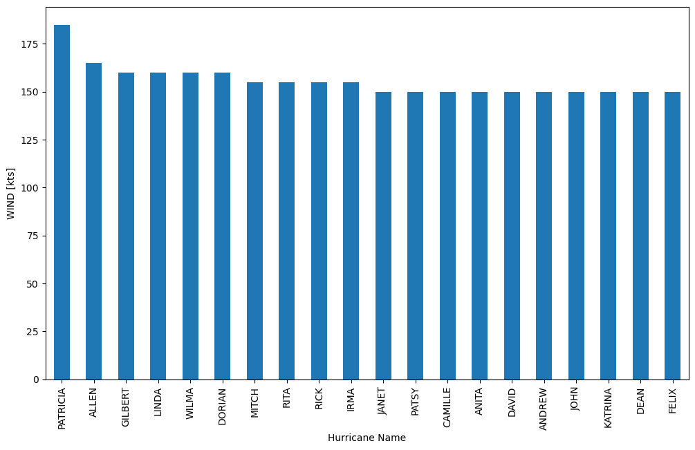
This bar plot provides a clear and informative representation of the top 20 hurricanes by maximum wind speed.

Plotting the count of all datapoints by Basin

df.groupby('BASIN').SID.count().sort_values().plot(kind='bar', logy=True, rot=0)
plt.show()

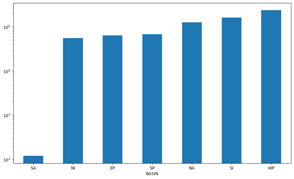
Code Explanation

1. We first need to group SID by BASIN

df.groupby('BASIN').SID

2. Now specify your aggregate function, here we will count() the number of SIDs per BASIN.

3. While note crucial, we usesort_values() so our Series is sorted from lowest to highest.

4. Finally we plot() - barplot, with logarithmic y axis, x labels rotation set to 0 degrees

Learning the keyword arguments for the plot() function is crucial. If you find this approach confusing, consider experimenting with various versions of this code to improve your understanding.

Making a hexbin of the location of datapoints in Latitude and Longitude

df.plot(kind='hexbin', x='LON', y='LAT', gridsize=200, cmap='coolwarm')
plt.show()

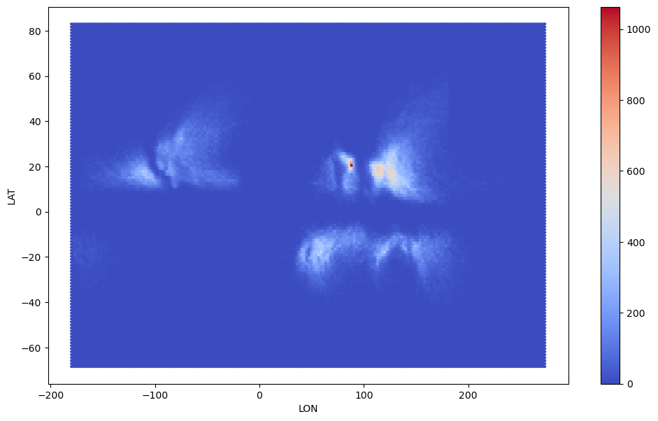
Code Explanation

A hexbin plot is a type of bivariate data visualization that enables us to examine the relationship between two variables simultaneously. In this context, we’re exploring how the frequency of storm data points varies concerning both latitude and longitude. Unlike a univariate analysis using a histogram, which would focus on just one variable at a time, a hexbin plot allows us to observe common locations where storm data points occur based on both latitude and longitude.

Notice that increasing the gridsize increases the resolution of your hexbin. The default will be 100 should you not specify.

For more details on the plot() function please review the official documentation.

To learn about more colour mappings, check out matplotlib documentation

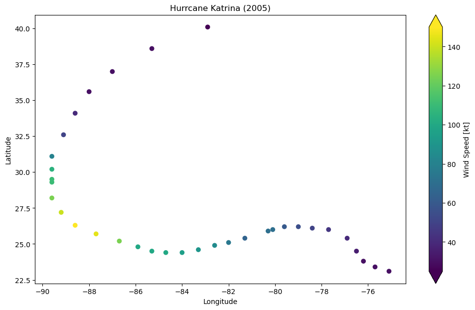
Finding Hurricane Katrina (from 2005) and plot its track as a scatter plot

katrina_filter = df['NAME']=='KATRINA'
time_2005_filter = df['ISO_TIME'].dt.year == 2005

katrina = df[katrina_filter & time_2005_filter]
katrina.head()

	SID	SEASON	NUMBER	BASIN	SUBBASIN	NAME	ISO_TIME	NATURE	LAT	LON	WIND	PRES
603763	2005236N23285	2005	61	NA	NA	KATRINA	2005-08-23 18:00:00	TS	23.1000	-75.1000	30.0	1008.0
603764	2005236N23285	2005	61	NA	NA	KATRINA	2005-08-23 21:00:00	TS	23.2476	-75.4049	NaN	NaN
603765	2005236N23285	2005	61	NA	NA	KATRINA	2005-08-24 00:00:00	TS	23.4000	-75.7000	30.0	1007.0
603766	2005236N23285	2005	61	NA	NA	KATRINA	2005-08-24 03:00:00	TS	23.5700	-75.9726	NaN	NaN
603767	2005236N23285	2005	61	NA	NA	KATRINA	2005-08-24 06:00:00	TS	23.8000	-76.2000	30.0	1007.0

There are various approaches to address this problem. Although each storm is identified by a unique SID, in this instance, we showcase slightly more advanced data filtering within Pandas.

1. Define the filter parameters

katrina_filter = df['NAME']=='KATRINA'
time_2005_filter = df['ISO_TIME'].dt.year == 2005

2. Apply the filters to the original DataFrame

katrina = df[katrina_filter & time_2005_filter]

plt.scatter(katrina.LON, katrina.LAT)
plt.show()

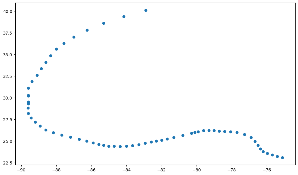
Do you think this plot could have been improved? Let’s try to improve this plot by using windspeed to colour points.

scatter = plt.scatter(katrina.LON, katrina.LAT, c=katrina.WIND)

cbar = plt.colorbar(scatter, extend='both')
cbar.set_label('Wind Speed [kt]') 

plt.xlabel('Longitude')
plt.ylabel('Latitude')
plt.title('Hurrcane Katrina (2005)')
plt.show()

Do not worry about adding maps to your points at this point, we will study this in more detail in a later tutorial.

Timeseries: Making time the index on your dataframe

df_time = df.set_index(['ISO_TIME'])

df_time.head()

	SID	SEASON	NUMBER	BASIN	SUBBASIN	NAME	NATURE	LAT	LON	WIND	PRES
ISO_TIME
1842-10-25 03:00:00	1842298N11080	1842	1	NI	BB	NaN	NR	10.9000	80.3000	NaN	NaN
1842-10-25 06:00:00	1842298N11080	1842	1	NI	BB	NaN	NR	10.8709	79.8265	NaN	NaN
1842-10-25 09:00:00	1842298N11080	1842	1	NI	BB	NaN	NR	10.8431	79.3524	NaN	NaN
1842-10-25 12:00:00	1842298N11080	1842	1	NI	BB	NaN	NR	10.8188	78.8772	NaN	NaN
1842-10-25 15:00:00	1842298N11080	1842	1	NI	BB	NaN	NR	10.8000	78.4000	NaN	NaN

Code Explanantion

Previously, we introduced the pd.DataFrame.set_index() function, which facilitates converting a column into the index of your dataset. In this case, we create a timeseries by assigning the ISO_TIME column to this position. Working with a timeseries expands the capabilities of Pandas and enhances the versatility of your analyses.

df_time = df.set_index(['ISO_TIME'])

Let’s take a look below

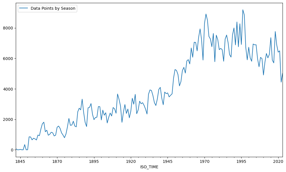
Plotting the count of all datapoints per year as a timeseries

We will use a new function for timeseries data, resample()

Notice that rule parameter values can be found in the Pandas Documentation

df_time.resample('Y').count().plot(y='SEASON', label='Data Points by Season')
plt.show()

Code Explanation

Another common operation is to change the resolution of a dataset by resampling in time. Pandas exposes this through the resample function. The resample periods are specified using pandas offset index syntax.

Here we resample the DataFrame by year then count the values for each year and finally plot the number of SEASON data points by year

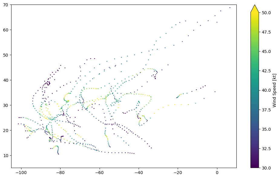
Plotting all tracks from the North Atlantic in 2005

Iterating through a GroupBy object

#applying filters
NA_basin_filter = df_time['BASIN']=='NA'
year_2005 = df_time.index.year == 2005


NA_2005 = df_time[NA_basin_filter & year_2005]
NA_2005.head()

	SID	SEASON	NUMBER	BASIN	SUBBASIN	NAME	NATURE	LAT	LON	WIND	PRES
ISO_TIME
2005-06-08 18:00:00	2005160N17276	2005	31	NA	CS	ARLENE	TS	16.9000	-84.0000	25.0	1004.0
2005-06-08 21:00:00	2005160N17276	2005	31	NA	CS	ARLENE	TS	17.1200	-83.9425	NaN	NaN
2005-06-09 00:00:00	2005160N17276	2005	31	NA	CS	ARLENE	TS	17.4000	-83.9000	30.0	1003.0
2005-06-09 03:00:00	2005160N17276	2005	31	NA	CS	ARLENE	TS	17.7775	-83.8850	NaN	NaN
2005-06-09 06:00:00	2005160N17276	2005	31	NA	CS	ARLENE	TS	18.2000	-83.9000	35.0	1003.0

NA_2005_grouped = NA_2005.groupby('NAME')
list(NA_2005_grouped.groups.keys())

['ALPHA',
 'ARLENE',
 'BETA',
 'BRET',
 'CINDY',
 'DELTA',
 'DENNIS',
 'EMILY',
 'EPSILON',
 'FRANKLIN',
 'GAMMA',
 'GERT',
 'HARVEY',
 'IRENE',
 'JOSE',
 'KATRINA',
 'LEE',
 'MARIA',
 'NATE',
 'OPHELIA',
 'PHILIPPE',
 'RITA',
 'STAN',
 'TAMMY',
 'VINCE',
 'WILMA',
 'ZETA']

As mentioned earlier, without an aggregate function, groupby() does not return a single DataFrame. Instead we have multiple DataFrames stored in a dictionary with the unique values of the grouped column being the keys.

Let’s take a look at DataFrame for the first key

for key, group in NA_2005_grouped:
    display(group.head())
    print(f'The key is "{key}"')
    break

	SID	SEASON	NUMBER	BASIN	SUBBASIN	NAME	NATURE	LAT	LON	WIND	PRES
ISO_TIME
2005-10-22 12:00:00	2005296N16293	2005	98	NA	CS	ALPHA	TS	15.8000	-67.5000	30.0	1007.0
2005-10-22 15:00:00	2005296N16293	2005	98	NA	CS	ALPHA	TS	16.1326	-67.9849	NaN	NaN
2005-10-22 18:00:00	2005296N16293	2005	98	NA	CS	ALPHA	TS	16.5000	-68.5000	35.0	1005.0
2005-10-22 21:00:00	2005296N16293	2005	98	NA	CS	ALPHA	TS	16.9150	-69.0573	NaN	NaN
2005-10-23 00:00:00	2005296N16293	2005	98	NA	CS	ALPHA	TS	17.3000	-69.6000	45.0	1000.0

The key is "ALPHA"

As you might imagine, we will need to plot each key-value pair on the same figure.

for key, group in NA_2005_grouped:
    plt.scatter(group.LON, group.LAT, c=group.WIND, s=1)
    
cbar = plt.colorbar(extend='max')
cbar.set_label('Wind Speed [kt]')

plt.xlim(-105,10)
plt.ylim(5,70)

plt.show()

Code Explanation

To access each key’s DataFrame, we loop through the groupby object:

for key, group in NA_2005_grouped

For each group, we create a scatter plot:

plt.scatter(group.LON, group.LAT, c=group.WIND, s=1)

This generates a plot for each key-value pair on the same figure. Now some final adjustments to improve plot clarity.

cbar = plt.colorbar(extend='max')
cbar.set_label('Wind Speed [kt]')

plt.xlim(-105,10)
plt.ylim(5,70)

plt.show()

Filtering timeseries: Only data since 1970 from the North Atlantic (“NA”) Basin

This dataframe will be used for the rest of the demostration

year_filter = df_time.index.year >= 1970

NA_1970 = df_time[NA_basin_filter & year_filter]

NA_1970.head()

	SID	SEASON	NUMBER	BASIN	SUBBASIN	NAME	NATURE	LAT	LON	WIND	PRES
ISO_TIME
1970-05-17 18:00:00	1970138N12281	1970	43	NA	CS	ALMA	TS	11.5000	-79.0000	25.0	NaN
1970-05-17 21:00:00	1970138N12281	1970	43	NA	CS	ALMA	TS	11.6475	-79.1400	NaN	NaN
1970-05-18 00:00:00	1970138N12281	1970	43	NA	CS	ALMA	TS	11.8000	-79.3000	25.0	NaN
1970-05-18 03:00:00	1970138N12281	1970	43	NA	CS	ALMA	TS	11.9575	-79.4925	NaN	NaN
1970-05-18 06:00:00	1970138N12281	1970	43	NA	CS	ALMA	TS	12.1000	-79.7000	25.0	NaN

Pandas demonstrates excellent built-in support for time operations, especially within the groupby() context. With datasets with a DateTimeIndex, grouping and resampling based on common time units becomes straoghtforward. In this case, we filtered our dataset tom include only years \(\ge1970\)

df_time.index.year >= 1970

Final Thoughts

Mastering Pandas is essential. Before moving on to the Xarray tutorial, take a moment to consolidate your understanding of the concepts you’ve learned. Many of these concepts will resurface in future lessons.