
Disclaimer: Kindly be aware that the questions and datasets featured in this tutorial were originally presented by Ryan Abernathy in “An Introduction to Earth and Environmental Data Science”.
Pandas Fundamentals with Earthquake Data#
Welcome to this practical tutorial on Pandas, here we will review pandas fundamentals, such as how to
Open csv files
Manipulate dataframe indexes
Parse date columns
Examine basic dataframe statistics
Manipulate text columns and extract values
Plot dataframe contents using
Bar charts
Histograms
Scatter plots
First, import Numpy, Pandas and Matplotlib and set the display options.
import pandas as pd
import numpy as np
from matplotlib import pyplot as plt
%matplotlib inline
Note: %matplotlib inline is a command specific to Jupyter Notebook and JupyterLab, to enable the inline plotting of graphs and visualizations. It is typically used to display these plots directly below the code cell in the notebook.
Data is in .csv format and downloaded from the USGS Earthquakes Database is available at:
http://www.ldeo.columbia.edu/~rpa/usgs_earthquakes_2014.csv
You can open this file directly with Pandas.
Using Pandas’ read_csv function directly on a URL to open it as a DataFrame#
#url for data
url = "http://www.ldeo.columbia.edu/~rpa/usgs_earthquakes_2014.csv"
#read file using pandas
data = pd.read_csv(url)
Pandas provides various methods for fetching and reading data depending on the file type. Here, , since the file is in .csv format, we will untilize the pd.read_csv() function and assign the resulting DataFrame to the variable data.
#display first 5 rows
data.head()
| time | latitude | longitude | depth | mag | magType | nst | gap | dmin | rms | net | id | updated | place | type | |
|---|---|---|---|---|---|---|---|---|---|---|---|---|---|---|---|
| 0 | 2014-01-31 23:53:37.000 | 60.252000 | -152.7081 | 90.20 | 1.10 | ml | NaN | NaN | NaN | 0.2900 | ak | ak11155107 | 2014-02-05T19:34:41.515Z | 26km S of Redoubt Volcano, Alaska | earthquake |
| 1 | 2014-01-31 23:48:35.452 | 37.070300 | -115.1309 | 0.00 | 1.33 | ml | 4.0 | 171.43 | 0.34200 | 0.0247 | nn | nn00436847 | 2014-02-01T01:35:09.000Z | 32km S of Alamo, Nevada | earthquake |
| 2 | 2014-01-31 23:47:24.000 | 64.671700 | -149.2528 | 7.10 | 1.30 | ml | NaN | NaN | NaN | 1.0000 | ak | ak11151142 | 2014-02-01T00:03:53.010Z | 12km NNW of North Nenana, Alaska | earthquake |
| 3 | 2014-01-31 23:30:54.000 | 63.188700 | -148.9575 | 96.50 | 0.80 | ml | NaN | NaN | NaN | 1.0700 | ak | ak11151135 | 2014-01-31T23:41:25.007Z | 22km S of Cantwell, Alaska | earthquake |
| 4 | 2014-01-31 23:30:52.210 | 32.616833 | -115.6925 | 10.59 | 1.34 | ml | 6.0 | 285.00 | 0.04321 | 0.2000 | ci | ci37171541 | 2014-02-01T00:13:20.107Z | 10km WNW of Progreso, Mexico | earthquake |
The pd.DataFrame.head() function returns the first 5 rows of a DataFrame. To display a different number of rows, an integer value can be provided within the function, such as data.head(10), which would provide the first 10 rows. Similarly, the pd.DataFrame.tail() function presents the last 5 rows by default, displaying the final rows of the DataFrame.
#data types and summaries

data.info()
<class 'pandas.core.frame.DataFrame'>
RangeIndex: 120108 entries, 0 to 120107
Data columns (total 15 columns):
 #   Column     Non-Null Count   Dtype
---  ------     --------------   -----
 0   time       120108 non-null  object
 1   latitude   120108 non-null  float64
 2   longitude  120108 non-null  float64
 3   depth      120107 non-null  float64
 4   mag        120065 non-null  float64
 5   magType    120065 non-null  object
 6   nst        59688 non-null   float64
 7   gap        94935 non-null   float64
 8   dmin       85682 non-null   float64
 9   rms        119716 non-null  float64
 10  net        120108 non-null  object
 11  id         120108 non-null  object
 12  updated    120108 non-null  object
 13  place      120108 non-null  object
 14  type       120108 non-null  object
dtypes: float64(8), object(7)
memory usage: 13.7+ MB
While we can onserve the first few rows of the data, it doesn’t provide comprehensive information about the entire DataFrame. For this Pandas offers the pd.DataFrame.info(). This function provies a basic summary of the DataFrame which includes counts of non-null values, data types, field names and other details.
You should have seen that the dates were not automatically parsed into datetime types. pd.read_csv() actucally provides options for dealing with this. Let’s take a look.
Re-Reading Data: Defining Date Columns and Index#
#read file using pandas
data = pd.read_csv(url, parse_dates=['time','updated'], index_col='id') #date cols specified and index col specified

#display first 5 rows
data.head()
| time | latitude | longitude | depth | mag | magType | nst | gap | dmin | rms | net | updated | place | type | |
|---|---|---|---|---|---|---|---|---|---|---|---|---|---|---|
| id | ||||||||||||||
| ak11155107 | 2014-01-31 23:53:37.000 | 60.252000 | -152.7081 | 90.20 | 1.10 | ml | NaN | NaN | NaN | 0.2900 | ak | 2014-02-05 19:34:41.515000+00:00 | 26km S of Redoubt Volcano, Alaska | earthquake |
| nn00436847 | 2014-01-31 23:48:35.452 | 37.070300 | -115.1309 | 0.00 | 1.33 | ml | 4.0 | 171.43 | 0.34200 | 0.0247 | nn | 2014-02-01 01:35:09+00:00 | 32km S of Alamo, Nevada | earthquake |
| ak11151142 | 2014-01-31 23:47:24.000 | 64.671700 | -149.2528 | 7.10 | 1.30 | ml | NaN | NaN | NaN | 1.0000 | ak | 2014-02-01 00:03:53.010000+00:00 | 12km NNW of North Nenana, Alaska | earthquake |
| ak11151135 | 2014-01-31 23:30:54.000 | 63.188700 | -148.9575 | 96.50 | 0.80 | ml | NaN | NaN | NaN | 1.0700 | ak | 2014-01-31 23:41:25.007000+00:00 | 22km S of Cantwell, Alaska | earthquake |
| ci37171541 | 2014-01-31 23:30:52.210 | 32.616833 | -115.6925 | 10.59 | 1.34 | ml | 6.0 | 285.00 | 0.04321 | 0.2000 | ci | 2014-02-01 00:13:20.107000+00:00 | 10km WNW of Progreso, Mexico | earthquake |
#display dataframe info
data.info()
<class 'pandas.core.frame.DataFrame'>
Index: 120108 entries, ak11155107 to ak11453389
Data columns (total 14 columns):
 #   Column     Non-Null Count   Dtype
---  ------     --------------   -----
 0   time       120108 non-null  datetime64[ns]
 1   latitude   120108 non-null  float64
 2   longitude  120108 non-null  float64
 3   depth      120107 non-null  float64
 4   mag        120065 non-null  float64
 5   magType    120065 non-null  object
 6   nst        59688 non-null   float64
 7   gap        94935 non-null   float64
 8   dmin       85682 non-null   float64
 9   rms        119716 non-null  float64
 10  net        120108 non-null  object
 11  updated    120108 non-null  datetime64[ns, UTC]
 12  place      120108 non-null  object
 13  type       120108 non-null  object
dtypes: datetime64[ns, UTC](1), datetime64[ns](1), float64(8), object(4)
memory usage: 13.7+ MB
By including the parse_dates argument of pd.read_csv and a list of datetime columns, we can automatically convert these fields at the time of loading the DataFrame.
Using describe to get the basic statistics of all the columns#
Note the highest and lowest magnitude of earthquakes in the databse.
#describe dataframe and transposing it to make it more readable
data.describe().T

# T - transpose dataframe
| count | mean | min | 25% | 50% | 75% | max | std | |
|---|---|---|---|---|---|---|---|---|
| time | 120108 | 2014-07-05 09:10:37.116720128 | 2014-01-01 00:01:16.610000 | 2014-04-08 03:43:10.768999936 | 2014-07-07 10:44:06.035000064 | 2014-09-30 23:36:40.595000064 | 2014-12-31 23:54:33.900000 | NaN |
| latitude | 120108.0 | 38.399579 | -73.462 | 34.228917 | 38.8053 | 53.8895 | 86.6514 | 21.938258 |
| longitude | 120108.0 | -99.961402 | -179.9989 | -147.742025 | -120.832 | -116.0681 | 179.998 | 82.996858 |
| depth | 120107.0 | 28.375029 | -9.9 | 4.1 | 9.2 | 22.88 | 697.36 | 62.215416 |
| mag | 120065.0 | 1.793958 | -0.97 | 0.82 | 1.4 | 2.4 | 8.2 | 1.343466 |
| nst | 59688.0 | 17.878284 | 0.0 | 8.0 | 14.0 | 22.0 | 365.0 | 14.911369 |
| gap | 94935.0 | 124.048978 | 9.0 | 74.0 | 107.0 | 155.0 | 356.4 | 68.518595 |
| dmin | 85682.0 | 0.893198 | 0.0 | 0.02076 | 0.07367 | 0.447 | 64.498 | 2.903966 |
| rms | 119716.0 | 0.358174 | 0.0 | 0.07 | 0.2 | 0.59 | 8.46 | 0.364046 |
The pd.DataFrame.describe() function offers a statistical summary of all fields of numeric type. This summary helps in understanding the distribution of our data, a crucial aspect of exploratory data analysis.
Use of the T attribute (transpose), it’s solely at your discretion and how you prefer to display the returned DataFrame. This option can be particularly useful in rendering high-dimensional DataFrames with few rows, making them more comprehensible.
Using nlargest to get the top 20 earthquakes by magnitude#
Review the documentation for pandas.Series.nlargest here
#display the top 20 earthquakes by mag
data.nlargest(20,'mag')
| time | latitude | longitude | depth | mag | magType | nst | gap | dmin | rms | net | updated | place | type | |
|---|---|---|---|---|---|---|---|---|---|---|---|---|---|---|
| id | ||||||||||||||
| usc000nzvd | 2014-04-01 23:46:47.260 | -19.6097 | -70.7691 | 25.00 | 8.2 | mww | NaN | 23.0 | 0.609 | 0.66 | us | 2015-07-30 16:24:51.223000+00:00 | 94km NW of Iquique, Chile | earthquake |
| usc000rki5 | 2014-06-23 20:53:09.700 | 51.8486 | 178.7352 | 109.00 | 7.9 | mww | NaN | 22.0 | 0.133 | 0.71 | us | 2015-04-18 21:54:08.699000+00:00 | 19km SE of Little Sitkin Island, Alaska | earthquake |
| usc000p27i | 2014-04-03 02:43:13.110 | -20.5709 | -70.4931 | 22.40 | 7.7 | mww | NaN | 44.0 | 1.029 | 0.82 | us | 2015-06-06 07:31:05.755000+00:00 | 53km SW of Iquique, Chile | earthquake |
| usc000phx5 | 2014-04-12 20:14:39.300 | -11.2701 | 162.1481 | 22.56 | 7.6 | mww | NaN | 13.0 | 2.828 | 0.71 | us | 2015-04-18 21:54:27.398000+00:00 | 93km SSE of Kirakira, Solomon Islands | earthquake |
| usb000pr89 | 2014-04-19 13:28:00.810 | -6.7547 | 155.0241 | 43.37 | 7.5 | mww | NaN | 16.0 | 3.820 | 1.25 | us | 2015-04-18 21:54:18.633000+00:00 | 70km SW of Panguna, Papua New Guinea | earthquake |
| usc000piqj | 2014-04-13 12:36:19.230 | -11.4633 | 162.0511 | 39.00 | 7.4 | mww | NaN | 17.0 | 2.885 | 1.00 | us | 2015-08-13 19:29:13.018000+00:00 | 112km S of Kirakira, Solomon Islands | earthquake |
| usb000slwn | 2014-10-14 03:51:34.460 | 12.5262 | -88.1225 | 40.00 | 7.3 | mww | NaN | 18.0 | 1.078 | 0.70 | us | 2015-08-13 19:35:02.679000+00:00 | 74km S of Intipuca, El Salvador | earthquake |
| usb000pq41 | 2014-04-18 14:27:24.920 | 17.3970 | -100.9723 | 24.00 | 7.2 | mww | NaN | 46.0 | 2.250 | 1.20 | us | 2015-08-13 19:30:39.599000+00:00 | 33km ESE of Petatlan, Mexico | earthquake |
| usc000pft9 | 2014-04-11 07:07:23.130 | -6.5858 | 155.0485 | 60.53 | 7.1 | mww | NaN | 21.0 | 3.729 | 0.88 | us | 2014-07-01 02:37:56+00:00 | 56km WSW of Panguna, Papua New Guinea | earthquake |
| usc000sxh8 | 2014-11-15 02:31:41.720 | 1.8929 | 126.5217 | 45.00 | 7.1 | mww | NaN | 18.0 | 1.397 | 0.71 | us | 2015-03-20 18:42:02.735000+00:00 | 154km NW of Kota Ternate, Indonesia | earthquake |
| usc000stdc | 2014-11-01 18:57:22.380 | -19.6903 | -177.7587 | 434.00 | 7.1 | mww | NaN | 13.0 | 4.415 | 0.84 | us | 2015-01-20 09:03:09.040000+00:00 | 144km NE of Ndoi Island, Fiji | earthquake |
| usb000sk6k | 2014-10-09 02:14:31.440 | -32.1082 | -110.8112 | 16.54 | 7.0 | mww | NaN | 22.0 | 5.127 | 0.43 | us | 2015-08-13 19:31:44.129000+00:00 | Southern East Pacific Rise | earthquake |
| usc000mnvj | 2014-02-12 09:19:49.060 | 35.9053 | 82.5864 | 10.00 | 6.9 | mww | NaN | 18.0 | 7.496 | 0.83 | us | 2015-01-30 23:03:45.902000+00:00 | 272km ESE of Hotan, China | earthquake |
| usc000nzwm | 2014-04-01 23:57:58.790 | -19.8927 | -70.9455 | 28.42 | 6.9 | mww | NaN | 119.0 | 0.828 | 0.93 | us | 2014-05-29 23:32:13+00:00 | 91km WNW of Iquique, Chile | earthquake |
| usb000r2hc | 2014-05-24 09:25:02.440 | 40.2893 | 25.3889 | 6.43 | 6.9 | mww | NaN | 25.0 | 0.402 | 0.67 | us | 2015-01-28 09:17:17.266000+00:00 | 22km SSW of Kamariotissa, Greece | earthquake |
| usc000rngj | 2014-06-29 07:52:55.170 | -55.4703 | -28.3669 | 8.00 | 6.9 | mww | NaN | 25.0 | 4.838 | 0.76 | us | 2014-09-26 11:49:45+00:00 | 154km NNW of Visokoi Island, | earthquake |
| usc000rkg5 | 2014-06-23 19:19:15.940 | -29.9772 | -177.7247 | 20.00 | 6.9 | mww | NaN | 35.0 | 0.751 | 0.99 | us | 2014-09-19 17:23:16+00:00 | 80km SSE of Raoul Island, New Zealand | earthquake |
| usb000ruzk | 2014-07-21 14:54:41.000 | -19.8015 | -178.4001 | 615.42 | 6.9 | mww | NaN | 15.0 | 3.934 | 0.96 | us | 2014-10-17 21:12:13+00:00 | 99km NNE of Ndoi Island, Fiji | earthquake |
| usc000rr6a | 2014-07-07 11:23:54.780 | 14.7240 | -92.4614 | 53.00 | 6.9 | mww | NaN | 51.0 | 0.263 | 1.38 | us | 2015-01-28 13:08:13.282000+00:00 | 4km W of Puerto Madero, Mexico | earthquake |
| usb000rzki | 2014-08-03 00:22:03.680 | 0.8295 | 146.1688 | 13.00 | 6.9 | mww | NaN | 12.0 | 6.393 | 0.93 | us | 2014-10-29 19:52:55+00:00 | Federated States of Micronesia region | earthquake |
The pd.Series.nlargest() function is straightforward and incredibly useful. It operates on a pd.Series (a single column) and retrieves the top \(n\) values. When applied within a DataFrame context, it allows us to extract the rows containing the \(n\) largest values from the specified column.
Examine the structure of the place column. The state / country information seems to be in there. How would you get it out?
Extracting the state or country and adding it a new column to the dataframe called country.#
Note that some of the “countries” are actually U.S. states.
#text cleaning

#if there is a comma then split, if not just use text

def extract_locations(text):
    """ This function parses strings, splitting them based on a comma
        Then checks the length resulting list is more than zero
        Then takes the last entry from the list
        Then checks if the last in the list or the original sting itself is in the list of states
        If yes it returns USA
        If not it returns the entity
        If the entity has no comma then it returns the original text

        Parameters:
            text: takes a string input of variable length
        Return:
            string output of country name
    """

    #list of states of the US from
    # https://gist.githubusercontent.com/norcal82/e4c7e8113f377db184bb/raw/87558bb70c5c149f357663061bc1b1ab96c90b7e/state_names.py
    state_names = ["Alaska", "Alabama", "Arkansas", "American Samoa", "Arizona", "California", "Colorado", "Connecticut", "District ",
                   "of Columbia", "Delaware", "Florida", "Georgia", "Guam", "Hawaii", "Iowa", "Idaho", "Illinois", "Indiana", "Kansas",
                   "Kentucky", "Louisiana", "Massachusetts", "Maryland", "Maine", "Michigan", "Minnesota", "Missouri", "Mississippi",
                   "Montana", "North Carolina", "North Dakota", "Nebraska", "New Hampshire", "New Jersey", "New Mexico", "Nevada",
                   "New York", "Ohio", "Oklahoma", "Oregon", "Pennsylvania", "Puerto Rico", "Rhode Island", "South Carolina",
                   "South Dakota", "Tennessee", "Texas", "Utah", "Virginia", "Virgin Islands", "Vermont", "Washington", "Wisconsin",
                   "West Virginia", "Wyoming"]


    parts = text.split(', ')
    if len(parts) > 0:
        entity = parts[-1]
        if entity in state_names or text in state_names:
            return "USA"
        return entity

    return np.nan
Although this function may initially seem complex, its logic is quite straightforward. Observe the pattern within the place column, where country names typically appear after the final comma, or there are no commas, and the country/place name is provided in full.
To extract the country, we split each place name at commas:
parts = text.split(', ')
We then select the last string in the created list. If commas aren’t present, then the first and last string will be the same:
entity = parts[-1]
Additionally, we need to consider whether the place name is a U.S. state or not. If it is, we should return “USA”; otherwise, we can simply return
entityas it won’t be a U.S. state:if entity in state_names or text in state_names: return "USA" return entity
While not absolutely necessary in this circumstance, it’s good practice to specify behavior if the data in
placedoes not meet the specified logic above. This is why the final return is:return np.nan
data['country'] = data['place'].apply(extract_locations)
data.head()
| time | latitude | longitude | depth | mag | magType | nst | gap | dmin | rms | net | updated | place | type | country | |
|---|---|---|---|---|---|---|---|---|---|---|---|---|---|---|---|
| id | |||||||||||||||
| ak11155107 | 2014-01-31 23:53:37.000 | 60.252000 | -152.7081 | 90.20 | 1.10 | ml | NaN | NaN | NaN | 0.2900 | ak | 2014-02-05 19:34:41.515000+00:00 | 26km S of Redoubt Volcano, Alaska | earthquake | USA |
| nn00436847 | 2014-01-31 23:48:35.452 | 37.070300 | -115.1309 | 0.00 | 1.33 | ml | 4.0 | 171.43 | 0.34200 | 0.0247 | nn | 2014-02-01 01:35:09+00:00 | 32km S of Alamo, Nevada | earthquake | USA |
| ak11151142 | 2014-01-31 23:47:24.000 | 64.671700 | -149.2528 | 7.10 | 1.30 | ml | NaN | NaN | NaN | 1.0000 | ak | 2014-02-01 00:03:53.010000+00:00 | 12km NNW of North Nenana, Alaska | earthquake | USA |
| ak11151135 | 2014-01-31 23:30:54.000 | 63.188700 | -148.9575 | 96.50 | 0.80 | ml | NaN | NaN | NaN | 1.0700 | ak | 2014-01-31 23:41:25.007000+00:00 | 22km S of Cantwell, Alaska | earthquake | USA |
| ci37171541 | 2014-01-31 23:30:52.210 | 32.616833 | -115.6925 | 10.59 | 1.34 | ml | 6.0 | 285.00 | 0.04321 | 0.2000 | ci | 2014-02-01 00:13:20.107000+00:00 | 10km WNW of Progreso, Mexico | earthquake | Mexico |
Let’s create a new column in the DataFrame.
Create a column in the DataFrame using the syntax
DataFrame['new_column']:data['country']
Populate the new column with data. In this case, we want to extract the country name from the
placecolumn. To achieve this, we need to apply a function to the data within the column.Pandasfacilitates this through thepd.DataFrame.apply()function, which takes a function as its argument:data['place'].apply(extract_locations)
You can also attempt this using Pandas text data functions.
Displaying each unique value from the new column#
Review the documentation for pandas.Series.unique here
#each unique value
data.country.unique()
array(['USA', 'Mexico', 'Papua New Guinea', 'New Zealand',
       'South of the Fiji Islands', 'British Virgin Islands', 'Canada',
       'Fiji', 'Antarctica', 'Chile', 'Indonesia', 'Solomon Islands',
       'Micronesia', 'Russia', 'Philippines', 'Bolivia', 'Greece',
       'Japan', 'Iran', 'Tonga', 'Wallis and Futuna', 'CA',
       'Carlsberg Ridge', 'Pakistan',
       'Off the west coast of northern Sumatra', 'Burma', 'China', 'Peru',
       'Off the east coast of the North Island of New Zealand',
       'Costa Rica', 'Reykjanes Ridge', 'East Timor',
       'Central East Pacific Rise', 'Mid-Indian Ridge', 'Japan region',
       'Northern Mariana Islands', 'El Salvador', 'Samoa',
       'Northern Mid-Atlantic Ridge', 'Taiwan', 'South Sandwich Islands',
       'Colombia', 'Dominican Republic', 'Argentina', 'Saint Helena',
       'West of Vancouver Island', 'Tanzania', 'Vanuatu',
       'Bosnia and Herzegovina', 'India', 'Southeast of Easter Island',
       'Serbia', 'Off the coast of Oregon', 'Nicaragua',
       'Republic of the Congo', 'Western Indian-Antarctic Ridge',
       'U.S. Virgin Islands', 'Southern East Pacific Rise', '',
       'Guatemala', 'Kyrgyzstan', 'Kuril Islands', 'Afghanistan',
       'Scotia Sea', 'West of Macquarie Island',
       'North of Ascension Island', 'New Caledonia', 'Saudi Arabia',
       'Southern Pacific Ocean', 'Romania', 'Italy',
       'Southern Mid-Atlantic Ridge', 'Panama', 'South Indian Ocean',
       'West Chile Rise', 'South of Panama', 'Albania', 'Haiti',
       'Ecuador', 'Tajikistan', 'Venezuela', 'North Indian Ocean',
       'Hungary', 'Central Mid-Atlantic Ridge', 'Christmas Island',
       'West of the Galapagos Islands', 'Bouvet Island', 'Greenland Sea',
       'South of Africa', 'Eritrea', 'Vanuatu region',
       'North of Svalbard', 'Sea of Okhotsk',
       '1km ENE of Quarry at VICTORVILLE', 'Turkmenistan',
       'East of Severnaya Zemlya', '1km NNE of Quarry at BORON',
       'Southeast Indian Ridge', 'Turkey',
       'British Indian Ocean Territory', 'Australia', 'Fiji region',
       'Southwest of Africa', '3km WSW of Quarry at CUSHENBURY', 'Cuba',
       'Guadeloupe', 'Azerbaijan', 'eastern Montana',
       'South Atlantic Ocean', 'Anguilla', 'Mauritania',
       'East of the North Island of New Zealand',
       'Chagos Archipelago region', 'Banda Sea', 'Easter Island region',
       'Comoros', 'Galapagos Triple Junction region', 'Honduras',
       'South of the Kermadec Islands', 'Davis Strait',
       'East of the Kuril Islands', 'Off the south coast of Australia',
       'Prince Edward Islands', 'Mongolia', 'Mauritius - Reunion region',
       'Drake Passage', 'Indian Ocean Triple Junction',
       'Prince Edward Islands region', 'Cape Verde', 'Yemen',
       'Owen Fracture Zone region', 'Spain', 'North Atlantic Ocean',
       'Algeria', 'Pacific-Antarctic Ridge', 'Mauritius',
       'Southwest Indian Ridge', 'Aruba', 'Svalbard and Jan Mayen',
       'United Kingdom', 'Crozet Islands region', 'Barbados',
       'Cook Islands', 'Bangladesh', 'South Sudan', 'Greenland',
       'Martinique', 'Balleny Islands region', 'Cyprus', 'South of Tonga',
       'Malaysia', 'North Korea', 'Off the coast of Central America',
       'Cayman Islands', 'Portugal', 'Ethiopia',
       'Azores-Cape St. Vincent Ridge', 'Uzbekistan', 'India region',
       'French Southern Territories', 'Poland',
       'South Georgia Island region', 'North of New Zealand', 'Egypt',
       'Morocco', 'Slovenia', 'East of the South Sandwich Islands',
       'Ascension Island region', 'western Montana',
       'East central Pacific Ocean', 'Timor Sea', 'West of Australia',
       'Labrador Sea', 'Somalia', 'Zambia', 'Saint Martin', 'Ukraine',
       'Southwest of Australia', 'Mariana Islands region',
       'Norwegian Sea', 'France', 'Gulf of Alaska',
       'Northwest of Australia', 'Montenegro', 'Bermuda', 'South Africa',
       'North of Severnaya Zemlya', 'Saint Kitts and Nevis', 'Iraq',
       'Bouvet Island region', 'North of Franz Josef Land', 'Laptev Sea',
       'Brazil', 'Southeast central Pacific Ocean',
       'South Georgia and the South Sandwich Islands',
       'Northern California', 'Central California', 'Czech Republic',
       'Mozambique Channel', 'Santa Cruz Islands region',
       'Macquarie Island region', 'Alaska Peninsula', 'Oman',
       'Azores Islands region', 'Off the coast of Ecuador',
       'Central Alaska', 'Macedonia', 'Southeastern Alaska',
       'Southern Alaska', 'Lebanon', 'northern Alaska', 'Jordan',
       'Southern California', 'Puerto Rico region', 'Djibouti',
       'Molucca Sea', 'Leeward Islands', 'Germany', 'south of Panama',
       'Celebes Sea', 'Iceland', 'Falkland Islands region',
       'Ecuador region', 'Vietnam', 'South of Alaska',
       'Philippine Islands region', 'western Texas',
       'northern Mid-Atlantic Ridge', 'Russia region', 'Thailand',
       'Peru-Ecuador border region', 'Jamaica', 'Kermadec Islands region',
       'north of Ascension Island', 'Tristan da Cunha region',
       'Western Australia', 'Tonga region', 'Palau region',
       'East of the Philippine Islands', 'southern Idaho', 'Kazakhstan',
       'south of the Aleutian Islands', 'South Sandwich Islands region',
       'western Xizang', 'Norway', 'South Shetland Islands',
       'Virgin Islands region', 'offshore Northern California',
       'South of Australia', 'Southwestern Atlantic Ocean',
       'Saint Eustatius and Saba ', 'Jersey',
       'Northern East Pacific Rise', 'Trinidad and Tobago', 'Burundi',
       'Niue', 'Dominica', 'Nepal',
       'Off the coast of Southeastern Alaska',
       'Federated States of Micronesia region', 'Bay of Bengal',
       'Barbuda', 'South Napa Earthquake', 'East of the Volcano Islands',
       'Syria', 'Uganda', 'Sweden', 'South of the Mariana Islands',
       'Mozambique', 'Saint Vincent and the Grenadines', 'Sudan',
       'Socotra region', 'French Polynesia', 'Palau',
       'Tennessee-Virginia border region',
       'Democratic Republic of the Congo', 'Bhutan', 'Angola',
       'Portugal region', 'Malawi', 'South of Tasmania',
       'Eastern Greenland', 'Kosovo', 'Saint Lucia',
       'Off the south coast of Northwest Africa', 'Sierra Leone'],
      dtype=object)
#number of unique country values
data.country.nunique()
286
Observe the difference between pd.Series.unique() and pd.Series.nunique(). To get a better idea, try
len(data.country.unique())
Note that the country column is still imperfect. There are methods to further clean this column using libraries such as SpaCy or NLTK but that is outside of the scope of this tutorial.
I recommend taking a look at a course in Information Retrieval or Natural Language Processing to gain further familiarity, if interested.
Filtering A Dataset: Magnitude 4 or Larger Earthquakes#
#filtering in pandas

filter = data['mag']>=4
magnitude_4_and_higher = data[filter]

magnitude_4_and_higher.head()
| time | latitude | longitude | depth | mag | magType | nst | gap | dmin | rms | net | updated | place | type | country | |
|---|---|---|---|---|---|---|---|---|---|---|---|---|---|---|---|
| id | |||||||||||||||
| usc000mqlp | 2014-01-31 23:08:03.660 | -4.9758 | 153.9466 | 110.18 | 4.2 | mb | NaN | 98.0 | 1.940 | 0.61 | us | 2014-04-08 01:43:19+00:00 | 115km ESE of Taron, Papua New Guinea | earthquake | Papua New Guinea |
| usc000mqln | 2014-01-31 22:54:32.970 | -28.1775 | -177.9058 | 95.84 | 4.3 | mb | NaN | 104.0 | 1.063 | 1.14 | us | 2014-04-08 01:43:19+00:00 | 120km N of Raoul Island, New Zealand | earthquake | New Zealand |
| usc000mqls | 2014-01-31 22:49:49.740 | -23.1192 | 179.1174 | 528.34 | 4.4 | mb | NaN | 80.0 | 5.439 | 0.95 | us | 2014-04-08 01:43:19+00:00 | South of the Fiji Islands | earthquake | South of the Fiji Islands |
| usc000mf1x | 2014-01-31 22:19:44.330 | 51.1569 | -178.0910 | 37.50 | 4.2 | mb | NaN | NaN | NaN | 0.83 | us | 2014-04-08 01:43:19+00:00 | 72km E of Amatignak Island, Alaska | earthquake | USA |
| usc000mqlm | 2014-01-31 21:56:44.320 | -4.8800 | 153.8434 | 112.66 | 4.3 | mb | NaN | 199.0 | 1.808 | 0.79 | us | 2014-04-08 01:43:19+00:00 | 100km ESE of Taron, Papua New Guinea | earthquake | Papua New Guinea |
Pandas simplifies the process of data filtering.
Define our filter criteria - earthquakes with a magnitude of 4 or higher:
filter = data['mag'] >= 4
This filter creates a boolean mask, marking
Truewhere themagis greater than or equal to \(4\).Apply the created filter to the data:
data[filter]
This operation selects all rows from the
dataDataFrame where thefilterevaluates toTrue. You can also create more intricate filters. For instance, try filtering earthquakes between magnitudes \(6\) and \(9\).Hint - take a look here
Making a bar chart of the top 5 locations with the most earthquakes from the filtered dataset
Location name on the x axis, Earthquake count on the y axis
Method one using nlargest()
# get value counts of
country_freq = magnitude_4_and_higher['country'].value_counts()

top_5 = country_freq.nlargest(5)

top_5.plot(kind='bar', grid=True)

plt.show()
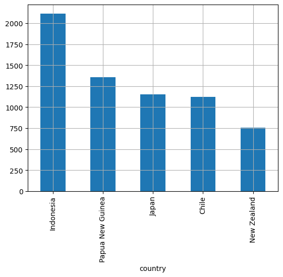
Pandas offers the pd.Series.value_counts() function, which generates an ordered series displaying counts for each unique value within a series or column.
Try executing:
magnitude_4_and_higher['country'].value_counts()
Additionally, Pandas seamlessly interfaces with Matplotlib through pd.DataFrame.plot(). This function allows us to specify the desired plot type and other keyword arguments, offering extensive customization options.
For example:
top_5.plot(kind='bar', grid=True)
Refer to the documentation here for more detailed information.
Getting familiar with this syntax is crucial as it’s extensively used in various data analysis and manipulation packages commonly utilized in scientific computing.es and research.
Method 2 using head()
# get value counts
country_freq = magnitude_4_and_higher['country'].value_counts()

#get top 5 from series suing head()
top_5 = country_freq.head()

#plot bar chart using matplotlib.pyplot.bar()
plt.bar(top_5.index, top_5)

#rotate the x labels 90 degrees
plt.xticks(rotation=90)

plt.grid(which='major')

plt.show()
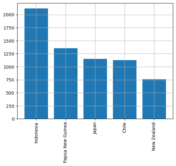
Notice the syntax variation when calling the Matplotlib.pyplot.bar() function directly instead of using pd.DataFrame.plot().
The pd.DataFrame.head() method could be utilized similarly to the first method. This plot showcases the adaptability of Pandas, highlighting that there’s no sole method to achieve an output. Experimenting with different methods will enhance your coding proficiency.
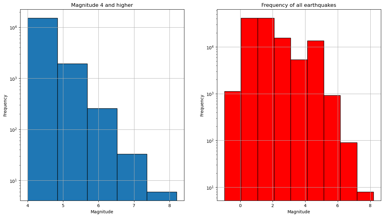
Making a histogram of the distribution of the Earthquake magnitudes#
For more information visit pandas.DataFrame.hist or matplotlib.pyplot.hist
#create figure
plt.figure(figsize=(15,8))

#create subplots
plt.subplot(1,2,1) #1 row, 2 cols and first position
#histogram, with ylog scale, grid and edges of bins in black
magnitude_4_and_higher['mag'].plot(kind='hist',logy=True, grid=True, edgecolor='black', bins=5)

#name x axis
plt.xlabel('Magnitude')

#name subplot
plt.title('Magnitude 4 and higher')

plt.subplot(1,2,2)
data['mag'].plot(kind='hist',logy=True, grid=True, color='red', edgecolor='black', bins=9)
plt.xlabel('Magnitude')
plt.title('Frequency of all earthquakes')

plt.show()
Let’s explore another effective method for creating subplots.
We can separate the figure and subplot creation steps:
# Create figure
plt.figure(figsize=(15, 8))

# Create the first subplot
plt.subplot(1, 2, 1)
# Subplot code

# Create the second subplot
plt.subplot(1, 2, 2)
# Subplot code
Here, we establish a \(1 \times 2\) subplot grid, specifying the location for the subsequent subplot as \(1\) and the next as \(2\).
Take note of the title creation for each plot compared to the methods used previously.
Additionally, a histogram is generated, showcasing various keyword arguments available in pd.DataFrame.plot():
data['mag'].plot(kind='hist', logy=True, grid=True, color='red', edgecolor='black', bins=9)
It’s crucial to emphasize the significance of reviewing the documentation for the pd.DataFrame.plot() function.
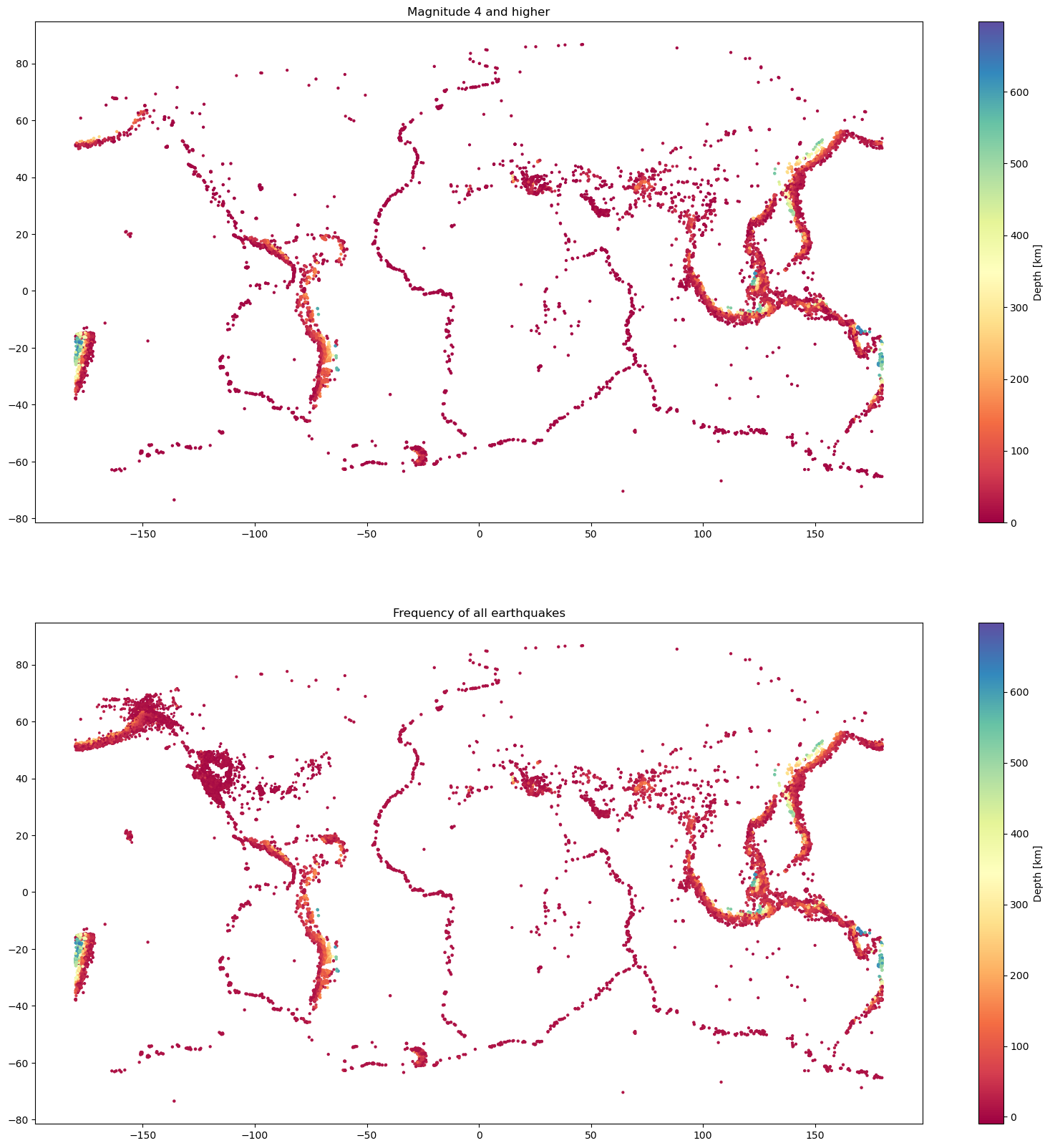
Visualising the locations of earthquakes with a scatterplot of their latitude and longitude#
Examine the code block below, try to note the purpose of each step.
#create figure
plt.figure(figsize=(20, 20))

#create subplots
plt.subplot(2,1,1)
#make scatter plot
scatter = plt.scatter(magnitude_4_and_higher.longitude,
                      magnitude_4_and_higher.latitude,
                      s=magnitude_4_and_higher.mag,
                      c=magnitude_4_and_higher.depth,
                     cmap='Spectral')
#create colorbar
cbar = plt.colorbar(scatter)
# Set colorbar label
cbar.set_label('Depth [km]')
#name subplot
plt.title('Magnitude 4 and higher')


#subplot 2
plt.subplot(2,1,2)
#make scatter plot
scatter = plt.scatter(data.longitude,
                      data.latitude,
                      s=data.mag,
                      c=data.depth,
                     cmap='Spectral')
#create colorbar
cbar = plt.colorbar(scatter) #format colorbar for 10^x)
# Set colorbar label
cbar.set_label('Depth [km]')
#name subplot
plt.title('Frequency of all earthquakes')

plt.show()
Did you understand how these plots were created?
Hint: Review the tutorial on Matplotlib.
Take a look matplotlib.pyplot for more cmap options. Try improving or changing aspects of the code above.
Final Thoughts#
By now, you should have acquired a foundational understanding of Pandas and its significance in data analysis and manipulation. Widely utilized in advanced scientific computing, Pandas offers extensive capabilities that we will delve into further in upcoming sections. Before progressing, ensure you comprehend and validate the calculations and transformations introduced in this chapter to solidify your grasp of the material.