
Python client#
The web interface (STAC Browser) discussed in the previous section is great for:
quickly exploring the catalog to see what data is available on the network
for examining the properties of various collections, and
for quickly getting access links to a small number of files.
If your analysis is limited to using selected data files, then you could hardcode the access links to those files that you obtained from the STAC Browser. However, often you might need several data files from a collection and manually searching for and copy-pasting the links to those files from the Browser into your notebooks is not feasible, and a programmatic approach becomes immediately desirable.
A more serious limitation of hardcoding access links from the web interface is that if the links for the data change, then your code will not function unless you manually update the code with the new links (again obtained from a manual search in the STAC Browser). This can lead to your code becoming less reproducible and can create problems for you down the line and problems for anyone with whom you’ve shared the code. For these reasons we recommend that you limit the usage of the web interface to the first two aforementioned use cases, and for accessing data links, you use the programmatic approach described here.
pystac-client#
The library that we will use to programmatically interact and query the Marble STAC catalog is called pystac-client. This is built on the robust pystac library for creating and reading STAC Catalogs,
and extends that by allowing the ability to work with a STAC API. We highly encourage you to look at the tutorials on the pystac-client
readthedocs page before proceeding further.
pystac-client comes installed in your Marble JupyterLab environments. If you are following along on a different platform,
you can install it per the instructions here.
Note
This tutorial will use the Marble platform’s CMIP6 data stored on the Red Oak node as an example.
Connecting to Marble STAC API#
The Red Oak node’s STAC API can be reached at http://redoak.cs.toronto.edu/stac. We start by importing the pystac_client library.
import pystac_client
Now, we use the Client.open function call to make a connection to the STAC API.
catalog = pystac_client.Client.open("http://redoak.cs.toronto.edu/stac")
type(catalog)
pystac_client.client.Client
That’s it! We’ve made a successful connection to the API. We now have a object named here catalog that we will use for all further interactions with the API.
Examining the Client object#
Before we get into searching for catalog items, let’s examine a few things that we can do with the Client object that we’ve created above.
Red Oak’s STAC endpoint contains various information about the catalog in JSON format, which has been copied here:
Caution
This content can be out of sync with the latest information on the API endpoint, this material is included here just for illustrative purposes.
{
  "type": "Catalog",
  "id": "stac-fastapi",
  "title": "Data Analytics for Canadian Climate Services STAC API",
  "description": "Searchable spatiotemporal metadata describing climate and Earth observation datasets.",
  "stac_version": "1.0.0",
  "conformsTo": [
    "https://api.stacspec.org/v1.0.0-rc.1/item-search#filter:basic-cql",
    "https://api.stacspec.org/v1.0.0-rc.1/collections",
    "https://api.stacspec.org/v1.0.0-rc.1/core",
    "http://www.opengis.net/spec/ogcapi-features-1/1.0/conf/core",
    "https://api.stacspec.org/v1.0.0-rc.1/item-search#filter",
    "https://api.stacspec.org/v1.0.0-rc.1/item-search#sort",
    "https://api.stacspec.org/v1.0.0-rc.1/item-search#fields",
    "http://www.opengis.net/spec/ogcapi-features-3/1.0/conf/features-filter",
    "https://api.stacspec.org/v1.0.0-rc.1/item-search#query",
    "https://api.stacspec.org/v1.0.0-rc.1/item-search#context",
    "https://api.stacspec.org/v1.0.0-rc.1/ogcapi-features",
    "https://api.stacspec.org/v1.0.0-rc.1/ogcapi-features/extensions/transaction",
    "http://www.opengis.net/spec/ogcapi-features-4/1.0/conf/simpletx",
    "http://www.opengis.net/spec/ogcapi-features-3/1.0/conf/filter",
    "http://www.opengis.net/spec/ogcapi-features-1/1.0/conf/geojson",
    "http://www.opengis.net/spec/ogcapi-features-1/1.0/conf/oas30",
    "https://api.stacspec.org/v1.0.0-rc.1/item-search#filter:cql-text",
    "https://api.stacspec.org/v1.0.0-rc.1/item-search"
  ],
  "links": [
    {
      "rel": "self",
      "type": "application/json",
      "href": "https://redoak.cs.toronto.edu/stac/"
    },
    {
      "rel": "root",
      "type": "application/json",
      "href": "https://redoak.cs.toronto.edu/stac/"
    },
    {
      "rel": "data",
      "type": "application/json",
      "href": "https://redoak.cs.toronto.edu/stac/collections"
    },
    {
      "rel": "conformance",
      "type": "application/json",
      "title": "STAC/WFS3 conformance classes implemented by this server",
      "href": "https://redoak.cs.toronto.edu/stac/conformance"
    },
    {
      "rel": "search",
      "type": "application/geo+json",
      "title": "STAC search",
      "href": "https://redoak.cs.toronto.edu/stac/search",
      "method": "GET"
    },
    {
      "rel": "search",
      "type": "application/geo+json",
      "title": "STAC search",
      "href": "https://redoak.cs.toronto.edu/stac/search",
      "method": "POST"
    },
    {
      "rel": "child",
      "type": "application/json",
      "title": "CMIP6",
      "href": "https://redoak.cs.toronto.edu/stac/collections/CMIP6_UofT"
    },
    {
      "rel": "service-desc",
      "type": "application/vnd.oai.openapi+json;version=3.0",
      "title": "OpenAPI service description",
      "href": "https://redoak.cs.toronto.edu/stac/api"
    },
    {
      "rel": "service-doc",
      "type": "text/html",
      "title": "OpenAPI service documentation",
      "href": "https://redoak.cs.toronto.edu/stac/api.html"
    }
  ],
  "stac_extensions": [
    "https://raw.githubusercontent.com/radiantearth/stac-api-spec/v1.0.0-rc.1/fragments/context/json-schema/schema.json"
  ]
}
All this information can be accessed using the Client object that we created. For instance, you can get the title and description of the API endpoint:
print(f"Catalog title        : {catalog.title}")
print(f"Catalog description  : {catalog.description}")
Catalog title        : Data Analytics for Canadian Climate Services STAC API
Catalog description  : Searchable spatiotemporal metadata describing climate and Earth observation datasets.
Information on the STAC extensions used and the conformance standards of the API can be accessed as:
print("STAC Extensions:")
for item in catalog.stac_extensions:
    print(item)

print("\nConformances:")
for item in catalog.extra_fields['conformsTo']:
    print(item)
STAC Extensions:
https://raw.githubusercontent.com/radiantearth/stac-api-spec/v1.0.0-rc.1/fragments/context/json-schema/schema.json

Conformances:
https://api.stacspec.org/v1.0.0-rc.1/item-search#filter:basic-cql
https://api.stacspec.org/v1.0.0-rc.1/collections
https://api.stacspec.org/v1.0.0-rc.1/core
http://www.opengis.net/spec/ogcapi-features-1/1.0/conf/core
https://api.stacspec.org/v1.0.0-rc.1/item-search#filter
https://api.stacspec.org/v1.0.0-rc.1/item-search#sort
https://api.stacspec.org/v1.0.0-rc.1/item-search#fields
http://www.opengis.net/spec/ogcapi-features-3/1.0/conf/features-filter
https://api.stacspec.org/v1.0.0-rc.1/item-search#query
https://api.stacspec.org/v1.0.0-rc.1/item-search#context
https://api.stacspec.org/v1.0.0-rc.1/ogcapi-features
https://api.stacspec.org/v1.0.0-rc.1/ogcapi-features/extensions/transaction
http://www.opengis.net/spec/ogcapi-features-4/1.0/conf/simpletx
http://www.opengis.net/spec/ogcapi-features-3/1.0/conf/filter
http://www.opengis.net/spec/ogcapi-features-1/1.0/conf/geojson
http://www.opengis.net/spec/ogcapi-features-1/1.0/conf/oas30
https://api.stacspec.org/v1.0.0-rc.1/item-search#filter:cql-text
https://api.stacspec.org/v1.0.0-rc.1/item-search
The links in the catalog can be accessed as:
catalog.get_links()
[<Link rel=self target=http://redoak.cs.toronto.edu/stac>,
 <Link rel=root target=https://redoak.cs.toronto.edu/stac/>,
 <Link rel=data target=https://redoak.cs.toronto.edu/stac/collections>,
 <Link rel=conformance target=https://redoak.cs.toronto.edu/stac/conformance>,
 <Link rel=search target=https://redoak.cs.toronto.edu/stac/search>,
 <Link rel=search target=https://redoak.cs.toronto.edu/stac/search>,
 <Link rel=child target=https://redoak.cs.toronto.edu/stac/collections/CMIP6_UofT>,
 <Link rel=service-desc target=https://redoak.cs.toronto.edu/stac/api>,
 <Link rel=service-doc target=https://redoak.cs.toronto.edu/stac/api.html>]
You can get a collection, for example the “CMIP6_UofT” collection as follows:
cmip6_uoft = catalog.get_collection("CMIP6_UofT")
type(cmip6_uoft)
pystac_client.collection_client.CollectionClient
You can also retrieve the URL to the STAC API, if you need:
catalog.self_href
'http://redoak.cs.toronto.edu/stac'
You can use the Client and CollectionClient object along with the methods shown above (and several others not shown here) to navigate the API programmatically. This is probably not something you want to do; it’s better to navigate the catalog using the STAC Browser. But this brief introduction is included here to show you how to use the Client object for more than just searching, which is the topic to which we now turn.
Searching for data#
Basic search operations#
To perform search, we will use the search function of the Client object. Details of the search functionality are exposed below via means of examples.
Example 1: A simple search to get all items in a “collection”.
search = catalog.search(
    collections=["CMIP6_UofT"],  # This means search for all items in the "CMIP6_UofT" collection.
)
# All information about the search we just performed is now in the 'search' object, which is
# of type pystac_client.item_search.ItemSearch.
print(f"'search' is an object of type: {type(search)}\n")
# We can count the number of items that were found as follows:
print(f"Search returned {len(search.item_collection())} items")
'search' is an object of type: <class 'pystac_client.item_search.ItemSearch'>

Search returned 6831 items
This example shows how easy it is to get all items belonging to a STAC collection on the Marble network. Note that this example does not show how to retrieve the individual items in the search result or get their access URLs, that is discussed in a later section.
Example 2: Let’s say you know the unique ID’s of the data items within a collection, and your objective is to get those data items (so that you can then get their access links). How do you do that?
Note
In our example, the ID for a CMIP6 item in the “CMIP6_UofT” collection is constructed using the following format:
{activity_id}_{institution_id}_{source_id}_{experiment_id}_{variant_label}_{table_id}_{variable_id}_{grid_label}
where, each item in parenthesis is a term from the CMIP6 Controlled Vocabulary.
search = catalog.search(
    collections=["CMIP6_UofT"],
    # Here, we are looking for the following two items
    ids=["CMIP_UCSB_E3SM-1-0_historical_r8i2p2f1_Amon_tas_gr", "CMIP_UCSB_E3SM-1-0_historical_r9i2p2f1_Amon_clt_gr"],
)

print(f"Search returned {len(search.item_collection())} items")
Search returned 2 items
Since we are seaching for two items, and since IDs on a STAC catalog have to be unique, we received two search results. Anything different would be wrong.
In Example 2, you may choose to omit the parameter
collectionparameter to the search since IDs are unique in a STAC catalog.
Advanced search operations#
The standard STAC implementation provides, by default, the ability to search on a few key fields that are common to all STAC data structures, such as “collections”, “ids”, “datetime” and bounding box (“bbox”) (see here). We saw how to use search the “collections” and “ids” field in the examples above.
More complex query operations are supported via means of STAC API extensions, namely, the Query and Filter extensions. Using the facilities provided by these extensions, you can search for items based on the values of their “properties”. The STAC implementation on Marble includes the Query and Filter extentions and thereby provides you the ability to construct more complex search requests.
Search using STAC API Query extension#
The “query” feature is used by structuring the search request as a (nested) dictionary and passing it to the query parameter of the same search function used above.
Example 3: In this example, we reproduce the results from Example 1, but this time by using the query feature.
search = catalog.search(
    query={"collection": {"eq": "CMIP6_UofT"}},
)

print(f"Search returned {len(search.item_collection())} items")
Search returned 6831 items
We see the number of items returned is identical to that which was found in Example 1, as it should. Let’s understand the data that we passed to the query paramter and what it means. The dictionary data for the search request was:
{"collection": {"eq": "CMIP6_UofT"}}
This says “apply the operation defined by the dictionary {"eq": "CMIP6_UofT"} to the collection field of the dataset”. The operation dictionary itself, specified as a name-value pair, means “apply an equality operation, i.e. ‘eq’, where the equality tests that the value is CMIP6_UofT”.
Now, let’s find all items in the “CMIP6_UofT” again, but this time instead of checking the value of the “collection” field, let’s check for the value of a propetry that only data in the “CMIP6_UofT” collection have:
search = catalog.search(
    # The property cmip6:mip_era is only present in the CMIP6_UofT collection, and all data in that collection
    # have this property value set to CMIP6
    query={"cmip6:mip_era": {"eq": "CMIP6"}},
)

print(f"Search returned {len(search.item_collection())} items")
Search returned 6831 items
As we see, the result is the same, which is expected. However trivial the above example, it illustrates a simple operation on a property of the data that you want. We’ll expand on this below.
Example 4: Now, get all items in the CMIP6_UofT collection that are of variable type “tas” (surface temperature according to the CMIP6 controlled vocabulary).
search = catalog.search(
    collections=["CMIP6_UofT"],
    query={"cmip6:variable_id": {"eq": "tas"}},
)

print(f"Search returned {len(search.item_collection())} items")
Search returned 571 items
In this example, our search request, encoded as a dictionary object says “find all items where the cmip6:variable_id field equals tas”. Note, the collection parameter is not strictly necessary in this case since the property cmip6:variable_id is only a property of data in the “CMIP6_UofT” collection. This property is unique, because it is defined by a STAC extension that is only applied to CMIP6 data.
There are several other properties that apply to multiple (or even all) collections. For instance, fields like datetime, start_datetime, end_datetime apply to all collection, so if you want to query for data files that are within a specific collection within a specific time range, then you’d have to also specify the collection name, either in the collection parameter as shown above, or as an additional component of the query sent to the query parameter.
In the next example, we see how to extend simple queries to include more that one operation.
Example 5: Extending our above query to add another query on the “cmip6:institution_id” property. Now our query is composed of two tests: the first test is on property “cmip6:variable_id”, the second one on property “cmip6:institution_id”, both tests check for equality with respoect to specific values.
search = catalog.search(
    collections=["CMIP6_UofT"],
    query={"cmip6:variable_id": {"eq": "tas"}, "cmip6:institution_id" : {"eq": "UCSB"}},
)

print(f"Search returned {len(search.item_collection())} items")
Search returned 20 items
Using the STAC API Filter extension#
The STAC community appears to be moving in the direction of preferring the filter extension compared to the query extension. From the Query extension’s main page:
It is recommended to implement the Filter Extension instead of the Query Extension. Filter Extension is more well-defined, more expressive, and uses the standardized CQL2 query language instead of the proprietary language defined here. There is no plan to deprecate this extension, but it is also unlikely to see any further refinement or changes.
Therefore, in this section of the tutorial, we provide a brief introduction to the Filter extension. The examples will implement the same searches as in the previous section, but this time the searches will be performed using the Filter extension. This feature is exposed in the search function of the Client object using the filter parameter.
Example 6: Implementing Example 4 using the Filter extension.
search = catalog.search(
    # collections=["CMIP6_UofT"],
    filter={"op": "eq", "args": [{"property": "cmip6:variable_id"}, "tas"]},
)

print(f"Search returned {len(search.item_collection())} items")
Search returned 571 items
Our search returned items, which is the same number of items we found using the Query extension in Example 4. Our search request, which is again structured as a dictionary object, is slightly different this time:
{
  "op": "eq",
  "args": [
    {
      "property": "cmip6:variable_id"
    },
    "tas"
  ]
}
The first name-value pair (NV pair) in the object is "op": "eq" which means that the operation is a test of equality. The details of that operation itself, i.e. which property to test on and what value to test against, are specified as the second NV pair "args": [...], whose key is appropriately named “args” to signify that it contains the arguments to the operation.
Example 7: Implementing Example 5 using the Filter extension.
search = catalog.search(
    collections=["CMIP6_UofT"],
    filter={
    "op" : "and",
    "args": [
      {
        "op": "eq",
        "args": [ { "property": "cmip6:variable_id" }, "tas" ]
      },
      {
        "op": "eq",
        "args" : [ { "property": "cmip6:institution_id" }, "UCSB" ]
      }
    ]
  },
)

print(f"Search returned {len(search.item_collection())} items")
Search returned 20 items
The search returned items, which is the same number that weas obtained using the Query extension in Example 5.
The structure of the request this time is more complex:
{
  "op": "and",
  "args": [
    {
      "op": "eq",
      "args": [
        {
          "property": "cmip6:variable_id"
        },
        "tas"
      ]
    },
    {
      "op": "eq",
      "args": [
        {
          "property": "cmip6:institution_id"
        },
        "UCSB"
      ]
    }
  ]
}
Retrieving information from search results#
So far we’ve focused on performing searches and understanding how many search results are returned. We haven’t yet looked at how we get information about the matched datasets, including but not limited to information on how to access them. This is what we focus on in this section.
First, let’s perform a sample search that we are going to use for the discussion in this section. The sample search is just Example 4:
search = catalog.search(
    collections=["CMIP6_UofT"],
    query={"cmip6:variable_id": {"eq": "tas"}},
)

print(f"Search returned {len(search.item_collection())} items")
Search returned 571 items
You can access all items in the search result using the item_collection() method of the pystac_client.item_search.ItemSearch object (which for us, is search)
limit = 10 # will limit printing to just 10 items
print(f"Listing the first {limit} items of a total {len(search.item_collection())} returned by the search:")
print(*search.item_collection()[:limit], sep="\n")
Listing the first 10 items of a total 571 returned by the search:
<Item id=CMIP_EC-Earth-Consortium_EC-Earth3_historical_r150i1p1f1_Amon_tas_gr>
<Item id=CMIP_EC-Earth-Consortium_EC-Earth3_historical_r149i1p1f1_Amon_tas_gr>
<Item id=CMIP_EC-Earth-Consortium_EC-Earth3_historical_r148i1p1f1_Amon_tas_gr>
<Item id=CMIP_EC-Earth-Consortium_EC-Earth3_historical_r147i1p1f1_Amon_tas_gr>
<Item id=CMIP_EC-Earth-Consortium_EC-Earth3_historical_r146i1p1f1_Amon_tas_gr>
<Item id=CMIP_EC-Earth-Consortium_EC-Earth3_historical_r145i1p1f1_Amon_tas_gr>
<Item id=CMIP_EC-Earth-Consortium_EC-Earth3_historical_r144i1p1f1_Amon_tas_gr>
<Item id=CMIP_EC-Earth-Consortium_EC-Earth3_historical_r143i1p1f1_Amon_tas_gr>
<Item id=CMIP_EC-Earth-Consortium_EC-Earth3_historical_r142i1p1f1_Amon_tas_gr>
<Item id=CMIP_EC-Earth-Consortium_EC-Earth3_historical_r141i1p1f1_Amon_tas_gr>
Let’s get one item from the list of all items for further exploration.
item = search.item_collection()[0]
print(type(item))
<class 'pystac.item.Item'>
The object “item”, which represents the first search item, is an object of type . We can get several types of information about this item using operations supported by pystac, as shown below:
You can get the item’s ID:
item.id
'CMIP_EC-Earth-Consortium_EC-Earth3_historical_r150i1p1f1_Amon_tas_gr'
If the object has a datetime value, then you can get that:
item.datetime
In this case, there is no output because there is no “datetime” value associated with the item. That is because there is no single “datetime” associated with CMIP6 data, instead it has a “start_datetime” and “end_datetime”. We can access those values as keys of the “properties” of the item:
item.properties['start_datetime'], item.properties['end_datetime']
('1970-01-16T12:00:00Z', '2014-12-16T12:00:00Z')
The item’s geometry and bounding box can be accessed as follows:
item.geometry
{'type': 'Polygon',
 'coordinates': [[[0, -89.46282196044922],
   [0, 89.46282196044922],
   [359.296875, 89.46282196044922],
   [359.296875, -89.46282196044922],
   [0, -89.46282196044922]]]}
item.bbox
[0.0, -89.46282196044922, 359.296875, 89.46282196044922]
A list containing JSON Schemas for the STAC extensions that the object provides can be accessed as:
item.stac_extensions
['https://raw.githubusercontent.com/TomAugspurger/cmip6/main/json-schema/schema.json',
 'https://stac-extensions.github.io/datacube/v2.2.0/schema.json']
Various links related to the item can be accessed as:
item.links
[<Link rel=collection target=https://redoak.cs.toronto.edu/stac/collections/CMIP6_UofT>,
 <Link rel=parent target=https://redoak.cs.toronto.edu/stac/collections/CMIP6_UofT>,
 <Link rel=root target=<Client id=stac-fastapi>>,
 <Link rel=self target=https://redoak.cs.toronto.edu/stac/collections/CMIP6_UofT/items/CMIP_EC-Earth-Consortium_EC-Earth3_historical_r150i1p1f1_Amon_tas_gr>,
 <Link rel=source target=https://redoak.cs.toronto.edu/twitcher/ows/proxy/thredds/fileServer/datasets/CMIP6/CMIP/EC-Earth-Consortium/EC-Earth3/historical/r150i1p1f1/Amon/tas/gr/v20200412/tas_Amon_EC-Earth3_historical_r150i1p1f1_gr_197001-201412.nc>]
The “properties” of the item can be accessed as shown below. This returns a dictionary, where the keys are various property names.
item.properties
{'cmip6:grid': 'T255L91-ORCA1L75',
 'cmip6:realm': ['atmos'],
 'cmip6:source': 'EC-Earth3 (2019): \naerosol: none\natmos: IFS cy36r4 (TL255, linearly reduced Gaussian grid equivalent to 512 x 256 longitude/latitude; 91 levels; top level 0.01 hPa)\natmosChem: none\nland: HTESSEL (land surface scheme built in IFS)\nlandIce: none\nocean: NEMO3.6 (ORCA1 tripolar primarily 1 deg with meridional refinement down to 1/3 degree in the tropics; 362 x 292 longitude/latitude; 75 levels; top grid cell 0-1 m)\nocnBgchem: none\nseaIce: LIM3',
 'end_datetime': '2014-12-16T12:00:00Z',
 'cmip6:license': 'CMIP6 model data produced by EC-Earth-Consortium is licensed under a Creative Commons Attribution-ShareAlike 4.0 International License (https://creativecommons.org/licenses). Consult https://pcmdi.llnl.gov/CMIP6/TermsOfUse for terms of use governing CMIP6 output, including citation requirements and proper acknowledgment. Further information about this data, including some limitations, can be found via the further_info_url (recorded as a global attribute in this file) and at http://www.ec-earth.org. The data producers and data providers make no warranty, either express or implied, including, but not limited to, warranties of merchantability and fitness for a particular purpose. All liabilities arising from the supply of the information (including any liability arising in negligence) are excluded to the fullest extent permitted by law.',
 'cmip6:mip_era': 'CMIP6',
 'cmip6:product': 'model-output',
 'cmip6:version': '',
 'cmip6:table_id': 'Amon',
 'cube:variables': {'tas': {'type': 'data',
   'unit': 'K',
   'dimensions': ['time', 'lat', 'lon'],
   'description': 'Near-Surface Air Temperature'},
  'height': {'type': 'auxiliary',
   'unit': 'm',
   'dimensions': [''],
   'description': 'height'},
  'lat_bnds': {'type': 'data',
   'unit': '',
   'dimensions': ['lat', 'bnds'],
   'description': ''},
  'lon_bnds': {'type': 'data',
   'unit': '',
   'dimensions': ['lon', 'bnds'],
   'description': ''},
  'time_bnds': {'type': 'data',
   'unit': '',
   'dimensions': ['time', 'bnds'],
   'description': ''}},
 'start_datetime': '1970-01-16T12:00:00Z',
 'cmip6:frequency': 'mon',
 'cmip6:source_id': 'EC-Earth3',
 'cube:dimensions': {'lat': {'axis': 'y',
   'type': 'spatial',
   'extent': [-89.46282196044922, 89.46282196044922],
   'description': 'projection_y_coordinate'},
  'lon': {'axis': 'x',
   'type': 'spatial',
   'extent': [0.0, 359.296875],
   'description': 'projection_x_coordinate'},
  'time': {'type': 'temporal',
   'extent': ['1970-01-16T12:00:00Z', '2014-12-16T12:00:00Z'],
   'description': 'time'}},
 'cmip6:experiment': 'all-forcing simulation of the recent past',
 'cmip6:grid_label': 'gr',
 'cmip6:Conventions': 'CF-1.7 CMIP-6.2',
 'cmip6:activity_id': 'CMIP',
 'cmip6:institution': 'AEMET, Spain; BSC, Spain; CNR-ISAC, Italy; DMI, Denmark; ENEA, Italy; FMI, Finland; Geomar, Germany; ICHEC, Ireland; ICTP, Italy; IDL, Portugal; IMAU, The Netherlands; IPMA, Portugal; KIT, Karlsruhe, Germany; KNMI, The Netherlands; Lund University, Sweden; Met Eireann, Ireland; NLeSC, The Netherlands; NTNU, Norway; Oxford University, UK; surfSARA, The Netherlands; SMHI, Sweden; Stockholm University, Sweden; Unite ASTR, Belgium; University College Dublin, Ireland; University of Bergen, Norway; University of Copenhagen, Denmark; University of Helsinki, Finland; University of Santiago de Compostela, Spain; Uppsala University, Sweden; Utrecht University, The Netherlands; Vrije Universiteit Amsterdam, the Netherlands; Wageningen University, The Netherlands. Mailing address: EC-Earth consortium, Rossby Center, Swedish Meteorological and Hydrological Institute/SMHI, SE-601 76 Norrkoping, Sweden',
 'cmip6:source_type': ['AOGCM'],
 'cmip6:tracking_id': '',
 'cmip6:variable_id': 'tas',
 'cmip6:creation_date': '2019-07-06T22:29:19Z',
 'cmip6:experiment_id': 'historical',
 'cmip6:forcing_index': 1,
 'cmip6:physics_index': 1,
 'cmip6:variant_label': 'r150i1p1f1',
 'cmip6:institution_id': 'EC-Earth-Consortium',
 'cmip6:sub_experiment': 'none',
 'cmip6:further_info_url': 'https://furtherinfo.es-doc.org/CMIP6.EC-Earth-Consortium.EC-Earth3.historical.none.r150i1p1f1',
 'cmip6:realization_index': 150,
 'cmip6:sub_experiment_id': 'none',
 'cmip6:data_specs_version': '01.00.30',
 'cmip6:nominal_resolution': '100 km',
 'cmip6:initialization_index': 1}
Finally, the assets, which provide various access routes, can be accessed as shown below. This returns a dictionary with keys representing the access mode available for that data.
item.assets
{'ISO': <Asset href=https://redoak.cs.toronto.edu/twitcher/ows/proxy/thredds/iso/datasets/CMIP6/CMIP/EC-Earth-Consortium/EC-Earth3/historical/r150i1p1f1/Amon/tas/gr/v20200412/tas_Amon_EC-Earth3_historical_r150i1p1f1_gr_197001-201412.nc>,
 'WCS': <Asset href=https://redoak.cs.toronto.edu/twitcher/ows/proxy/thredds/wcs/datasets/CMIP6/CMIP/EC-Earth-Consortium/EC-Earth3/historical/r150i1p1f1/Amon/tas/gr/v20200412/tas_Amon_EC-Earth3_historical_r150i1p1f1_gr_197001-201412.nc>,
 'WMS': <Asset href=https://redoak.cs.toronto.edu/twitcher/ows/proxy/thredds/wms/datasets/CMIP6/CMIP/EC-Earth-Consortium/EC-Earth3/historical/r150i1p1f1/Amon/tas/gr/v20200412/tas_Amon_EC-Earth3_historical_r150i1p1f1_gr_197001-201412.nc>,
 'NcML': <Asset href=https://redoak.cs.toronto.edu/twitcher/ows/proxy/thredds/ncml/datasets/CMIP6/CMIP/EC-Earth-Consortium/EC-Earth3/historical/r150i1p1f1/Amon/tas/gr/v20200412/tas_Amon_EC-Earth3_historical_r150i1p1f1_gr_197001-201412.nc>,
 'UDDC': <Asset href=https://redoak.cs.toronto.edu/twitcher/ows/proxy/thredds/uddc/datasets/CMIP6/CMIP/EC-Earth-Consortium/EC-Earth3/historical/r150i1p1f1/Amon/tas/gr/v20200412/tas_Amon_EC-Earth3_historical_r150i1p1f1_gr_197001-201412.nc>,
 'OpenDAP': <Asset href=https://redoak.cs.toronto.edu/twitcher/ows/proxy/thredds/dodsC/datasets/CMIP6/CMIP/EC-Earth-Consortium/EC-Earth3/historical/r150i1p1f1/Amon/tas/gr/v20200412/tas_Amon_EC-Earth3_historical_r150i1p1f1_gr_197001-201412.nc>,
 'HTTPServer': <Asset href=https://redoak.cs.toronto.edu/twitcher/ows/proxy/thredds/fileServer/datasets/CMIP6/CMIP/EC-Earth-Consortium/EC-Earth3/historical/r150i1p1f1/Amon/tas/gr/v20200412/tas_Amon_EC-Earth3_historical_r150i1p1f1_gr_197001-201412.nc>,
 'NetcdfSubset': <Asset href=https://redoak.cs.toronto.edu/twitcher/ows/proxy/thredds/ncss/datasets/CMIP6/CMIP/EC-Earth-Consortium/EC-Earth3/historical/r150i1p1f1/Amon/tas/gr/v20200412/tas_Amon_EC-Earth3_historical_r150i1p1f1_gr_197001-201412.nc>}
Let’s say you want to open the data remotely via the “OpenDAP” protocol, and you want the URL for that. You can get that by:
item.assets['OpenDAP'].href
'https://redoak.cs.toronto.edu/twitcher/ows/proxy/thredds/dodsC/datasets/CMIP6/CMIP/EC-Earth-Consortium/EC-Earth3/historical/r150i1p1f1/Amon/tas/gr/v20200412/tas_Amon_EC-Earth3_historical_r150i1p1f1_gr_197001-201412.nc'
Similarly, if you wanted to download the data to your local device, you want to use the “HTTPServer” protocol, so you’d do:
item.assets['HTTPServer'].href
'https://redoak.cs.toronto.edu/twitcher/ows/proxy/thredds/fileServer/datasets/CMIP6/CMIP/EC-Earth-Consortium/EC-Earth3/historical/r150i1p1f1/Amon/tas/gr/v20200412/tas_Amon_EC-Earth3_historical_r150i1p1f1_gr_197001-201412.nc'
The above few lines of code show how to access information about a STAC item (here, in our object named “item”) using the abstractions provided by the pystac.item.Item class. If you wanted to just inspect the raw JSON representation of the STAC object you could do:
item.to_dict()
{'type': 'Feature',
 'stac_version': '1.0.0',
 'id': 'CMIP_EC-Earth-Consortium_EC-Earth3_historical_r150i1p1f1_Amon_tas_gr',
 'properties': {'cmip6:grid': 'T255L91-ORCA1L75',
  'cmip6:realm': ['atmos'],
  'cmip6:source': 'EC-Earth3 (2019): \naerosol: none\natmos: IFS cy36r4 (TL255, linearly reduced Gaussian grid equivalent to 512 x 256 longitude/latitude; 91 levels; top level 0.01 hPa)\natmosChem: none\nland: HTESSEL (land surface scheme built in IFS)\nlandIce: none\nocean: NEMO3.6 (ORCA1 tripolar primarily 1 deg with meridional refinement down to 1/3 degree in the tropics; 362 x 292 longitude/latitude; 75 levels; top grid cell 0-1 m)\nocnBgchem: none\nseaIce: LIM3',
  'end_datetime': '2014-12-16T12:00:00Z',
  'cmip6:license': 'CMIP6 model data produced by EC-Earth-Consortium is licensed under a Creative Commons Attribution-ShareAlike 4.0 International License (https://creativecommons.org/licenses). Consult https://pcmdi.llnl.gov/CMIP6/TermsOfUse for terms of use governing CMIP6 output, including citation requirements and proper acknowledgment. Further information about this data, including some limitations, can be found via the further_info_url (recorded as a global attribute in this file) and at http://www.ec-earth.org. The data producers and data providers make no warranty, either express or implied, including, but not limited to, warranties of merchantability and fitness for a particular purpose. All liabilities arising from the supply of the information (including any liability arising in negligence) are excluded to the fullest extent permitted by law.',
  'cmip6:mip_era': 'CMIP6',
  'cmip6:product': 'model-output',
  'cmip6:version': '',
  'cmip6:table_id': 'Amon',
  'cube:variables': {'tas': {'type': 'data',
    'unit': 'K',
    'dimensions': ['time', 'lat', 'lon'],
    'description': 'Near-Surface Air Temperature'},
   'height': {'type': 'auxiliary',
    'unit': 'm',
    'dimensions': [''],
    'description': 'height'},
   'lat_bnds': {'type': 'data',
    'unit': '',
    'dimensions': ['lat', 'bnds'],
    'description': ''},
   'lon_bnds': {'type': 'data',
    'unit': '',
    'dimensions': ['lon', 'bnds'],
    'description': ''},
   'time_bnds': {'type': 'data',
    'unit': '',
    'dimensions': ['time', 'bnds'],
    'description': ''}},
  'start_datetime': '1970-01-16T12:00:00Z',
  'cmip6:frequency': 'mon',
  'cmip6:source_id': 'EC-Earth3',
  'cube:dimensions': {'lat': {'axis': 'y',
    'type': 'spatial',
    'extent': [-89.46282196044922, 89.46282196044922],
    'description': 'projection_y_coordinate'},
   'lon': {'axis': 'x',
    'type': 'spatial',
    'extent': [0.0, 359.296875],
    'description': 'projection_x_coordinate'},
   'time': {'type': 'temporal',
    'extent': ['1970-01-16T12:00:00Z', '2014-12-16T12:00:00Z'],
    'description': 'time'}},
  'cmip6:experiment': 'all-forcing simulation of the recent past',
  'cmip6:grid_label': 'gr',
  'cmip6:Conventions': 'CF-1.7 CMIP-6.2',
  'cmip6:activity_id': 'CMIP',
  'cmip6:institution': 'AEMET, Spain; BSC, Spain; CNR-ISAC, Italy; DMI, Denmark; ENEA, Italy; FMI, Finland; Geomar, Germany; ICHEC, Ireland; ICTP, Italy; IDL, Portugal; IMAU, The Netherlands; IPMA, Portugal; KIT, Karlsruhe, Germany; KNMI, The Netherlands; Lund University, Sweden; Met Eireann, Ireland; NLeSC, The Netherlands; NTNU, Norway; Oxford University, UK; surfSARA, The Netherlands; SMHI, Sweden; Stockholm University, Sweden; Unite ASTR, Belgium; University College Dublin, Ireland; University of Bergen, Norway; University of Copenhagen, Denmark; University of Helsinki, Finland; University of Santiago de Compostela, Spain; Uppsala University, Sweden; Utrecht University, The Netherlands; Vrije Universiteit Amsterdam, the Netherlands; Wageningen University, The Netherlands. Mailing address: EC-Earth consortium, Rossby Center, Swedish Meteorological and Hydrological Institute/SMHI, SE-601 76 Norrkoping, Sweden',
  'cmip6:source_type': ['AOGCM'],
  'cmip6:tracking_id': '',
  'cmip6:variable_id': 'tas',
  'cmip6:creation_date': '2019-07-06T22:29:19Z',
  'cmip6:experiment_id': 'historical',
  'cmip6:forcing_index': 1,
  'cmip6:physics_index': 1,
  'cmip6:variant_label': 'r150i1p1f1',
  'cmip6:institution_id': 'EC-Earth-Consortium',
  'cmip6:sub_experiment': 'none',
  'cmip6:further_info_url': 'https://furtherinfo.es-doc.org/CMIP6.EC-Earth-Consortium.EC-Earth3.historical.none.r150i1p1f1',
  'cmip6:realization_index': 150,
  'cmip6:sub_experiment_id': 'none',
  'cmip6:data_specs_version': '01.00.30',
  'cmip6:nominal_resolution': '100 km',
  'cmip6:initialization_index': 1,
  'datetime': None},
 'geometry': {'type': 'Polygon',
  'coordinates': [[[0, -89.46282196044922],
    [0, 89.46282196044922],
    [359.296875, 89.46282196044922],
    [359.296875, -89.46282196044922],
    [0, -89.46282196044922]]]},
 'links': [{'rel': 'collection',
   'href': 'https://redoak.cs.toronto.edu/stac/collections/CMIP6_UofT',
   'type': 'application/json'},
  {'rel': 'parent',
   'href': 'https://redoak.cs.toronto.edu/stac/collections/CMIP6_UofT',
   'type': 'application/json'},
  {'rel': <RelType.ROOT: 'root'>,
   'href': 'http://redoak.cs.toronto.edu/stac',
   'type': <MediaType.JSON: 'application/json'>,
   'title': 'Data Analytics for Canadian Climate Services STAC API'},
  {'rel': 'self',
   'href': 'https://redoak.cs.toronto.edu/stac/collections/CMIP6_UofT/items/CMIP_EC-Earth-Consortium_EC-Earth3_historical_r150i1p1f1_Amon_tas_gr',
   'type': 'application/geo+json'},
  {'rel': 'source',
   'href': 'https://redoak.cs.toronto.edu/twitcher/ows/proxy/thredds/fileServer/datasets/CMIP6/CMIP/EC-Earth-Consortium/EC-Earth3/historical/r150i1p1f1/Amon/tas/gr/v20200412/tas_Amon_EC-Earth3_historical_r150i1p1f1_gr_197001-201412.nc',
   'type': 'application/x-netcdf',
   'title': 'datasets/CMIP6/CMIP/EC-Earth-Consortium/EC-Earth3/historical/r150i1p1f1/Amon/tas/gr/v20200412/tas_Amon_EC-Earth3_historical_r150i1p1f1_gr_197001-201412.nc'}],
 'assets': {'ISO': {'href': 'https://redoak.cs.toronto.edu/twitcher/ows/proxy/thredds/iso/datasets/CMIP6/CMIP/EC-Earth-Consortium/EC-Earth3/historical/r150i1p1f1/Amon/tas/gr/v20200412/tas_Amon_EC-Earth3_historical_r150i1p1f1_gr_197001-201412.nc',
   'type': '',
   'roles': []},
  'WCS': {'href': 'https://redoak.cs.toronto.edu/twitcher/ows/proxy/thredds/wcs/datasets/CMIP6/CMIP/EC-Earth-Consortium/EC-Earth3/historical/r150i1p1f1/Amon/tas/gr/v20200412/tas_Amon_EC-Earth3_historical_r150i1p1f1_gr_197001-201412.nc',
   'type': 'application/xml',
   'roles': ['data']},
  'WMS': {'href': 'https://redoak.cs.toronto.edu/twitcher/ows/proxy/thredds/wms/datasets/CMIP6/CMIP/EC-Earth-Consortium/EC-Earth3/historical/r150i1p1f1/Amon/tas/gr/v20200412/tas_Amon_EC-Earth3_historical_r150i1p1f1_gr_197001-201412.nc',
   'type': 'application/xml',
   'roles': ['visual']},
  'NcML': {'href': 'https://redoak.cs.toronto.edu/twitcher/ows/proxy/thredds/ncml/datasets/CMIP6/CMIP/EC-Earth-Consortium/EC-Earth3/historical/r150i1p1f1/Amon/tas/gr/v20200412/tas_Amon_EC-Earth3_historical_r150i1p1f1_gr_197001-201412.nc',
   'type': '',
   'roles': []},
  'UDDC': {'href': 'https://redoak.cs.toronto.edu/twitcher/ows/proxy/thredds/uddc/datasets/CMIP6/CMIP/EC-Earth-Consortium/EC-Earth3/historical/r150i1p1f1/Amon/tas/gr/v20200412/tas_Amon_EC-Earth3_historical_r150i1p1f1_gr_197001-201412.nc',
   'type': '',
   'roles': []},
  'OpenDAP': {'href': 'https://redoak.cs.toronto.edu/twitcher/ows/proxy/thredds/dodsC/datasets/CMIP6/CMIP/EC-Earth-Consortium/EC-Earth3/historical/r150i1p1f1/Amon/tas/gr/v20200412/tas_Amon_EC-Earth3_historical_r150i1p1f1_gr_197001-201412.nc',
   'type': 'text/html',
   'roles': ['data']},
  'HTTPServer': {'href': 'https://redoak.cs.toronto.edu/twitcher/ows/proxy/thredds/fileServer/datasets/CMIP6/CMIP/EC-Earth-Consortium/EC-Earth3/historical/r150i1p1f1/Amon/tas/gr/v20200412/tas_Amon_EC-Earth3_historical_r150i1p1f1_gr_197001-201412.nc',
   'type': 'application/x-netcdf',
   'roles': ['data']},
  'NetcdfSubset': {'href': 'https://redoak.cs.toronto.edu/twitcher/ows/proxy/thredds/ncss/datasets/CMIP6/CMIP/EC-Earth-Consortium/EC-Earth3/historical/r150i1p1f1/Amon/tas/gr/v20200412/tas_Amon_EC-Earth3_historical_r150i1p1f1_gr_197001-201412.nc',
   'type': 'application/x-netcdf',
   'roles': ['data']}},
 'bbox': [0.0, -89.46282196044922, 359.296875, 89.46282196044922],
 'stac_extensions': ['https://raw.githubusercontent.com/TomAugspurger/cmip6/main/json-schema/schema.json',
  'https://stac-extensions.github.io/datacube/v2.2.0/schema.json'],
 'collection': 'CMIP6_UofT'}
The raw JSON can be difficult to interpret in this format, so a better way is to use the JSON rendering capability of the IPython library as follows:
import IPython.display
IPython.display.JSON(item.to_dict())
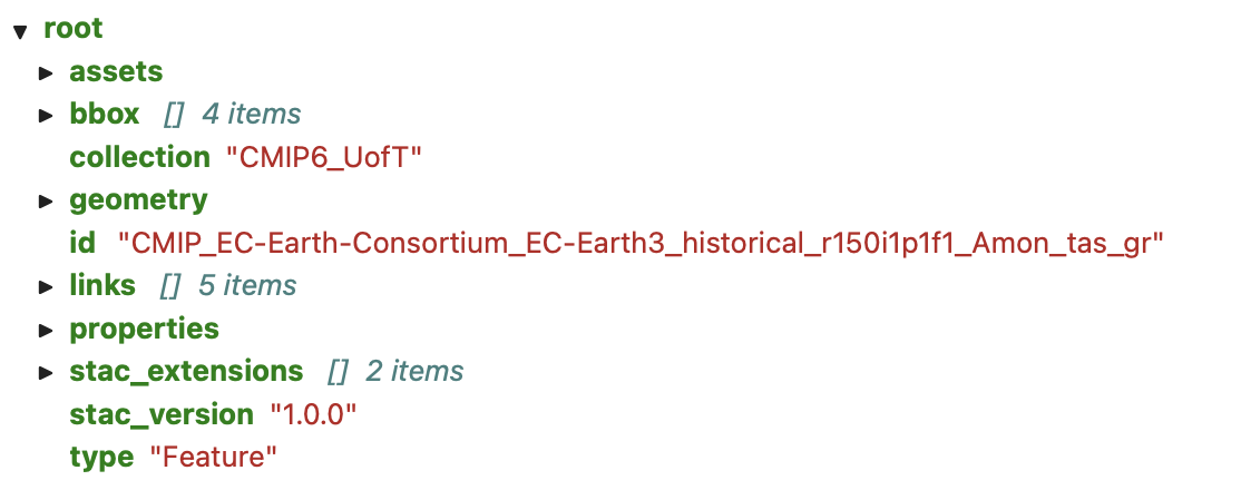
This presents the same information but in an interactive format where you can fold and expand the various elements of the JSON data to make the information easier to navigate.
Example workflow#
A simplified example that shows how to retrieve information about data of interest and how to incorporate it into your workflow is shown below:
# This is my special workflow involving the surface temperature variable.

# 1. First make my imports
import pystac_client
import xarray as xr

# 2. Open a link to the catalog
catalog = pystac_client.Client.open("http://redoak.cs.toronto.edu/stac")

# 3. Now, search for the data you want
search = catalog.search(
    collections=["CMIP6_UofT"],
    query={"cmip6:variable_id": {"eq": "tas"}},
)

num_found = len(search.item_collection())
print(f"Search returned {num_found} items")

# 4. Now open each file and do some calculation

for item in search.item_collection():
    print(f"Now processing: {item.id}")
    print("Some relevant info about this item: ")
    print(f"   CMIP6 Model ID : {item.properties['cmip6:source_id']}")
    print(f"   Variant label  : {item.properties['cmip6:variant_label']}")
    opendap_url = item.assets["OpenDAP"].href
    ds = xr.open_dataset(opendap_url)
    ...
    # Do analysis
    ds.close()